


















Lesson 14 of 45 · Transformers
Tests, Regulation and Efficiency
Find transformer parameters with open-circuit and short-circuit tests, compute voltage regulation and efficiency, and learn why maximum efficiency occurs where copper loss equals core loss.
You will rarely get the numbers for an equivalent circuit from a design drawing. You measure them. Two simple tests, one with the secondary open and one with it shorted, supply all the parameters with only a small amount of power, even for a transformer rated at many megavolt-amperes. From those parameters you can predict how the secondary voltage falls under load and how efficient the transformer is at any load and power factor.
What you will learn
- How to run and interpret the open-circuit and short-circuit tests.
- How to compute voltage regulation for lagging and leading loads.
- How to compute efficiency, the load of maximum efficiency and all-day efficiency.
Key terms
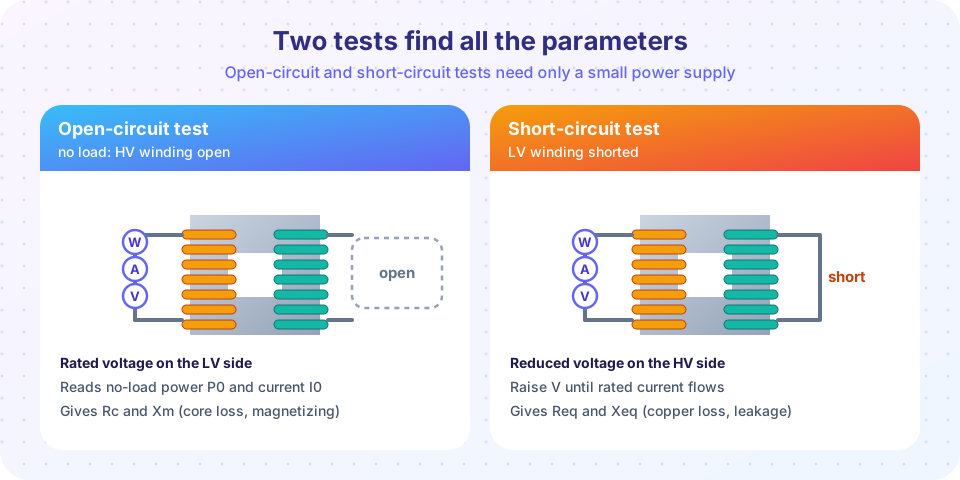
Open-circuit (no-load) test: rated voltage on one winding, the other open. Gives the core loss and magnetizing branch.
Short-circuit test: a reduced voltage on one winding, the other shorted, raised until rated current flows. Gives copper loss and the series impedance.
Voltage regulation: the relative change of the secondary voltage from no load to full load at a given power factor.
All-day efficiency: the ratio of energy out to energy in over 24 hours.
The open-circuit test
Apply rated voltage V0 to the low-voltage winding (convenient, because the voltage is lower and the supply is easy to find) and leave the other winding open. Measure the input voltage, current and power. Only the shunt branch carries current, and because the no-load current is small, the copper loss is negligible. So the wattmeter reads the core loss P0 = Pc.
cos φ0 = P0 / (V0 I0)
Ic = I0 cos φ0     Im = I0 sin φ0
Rc = V0 / Ic = V0² / P0      Xm = V0 / Im
Worked example. 10 kVA, 2000/200 V. Test on the 200 V side: V0 = 200 V, I0 = 1.2 A, P0 = 90 W.
cos φ0 = 90 / (200 × 1.2) = 0.375Ic = 0.45 A,Im = √(1.2² − 0.45²) = 1.11 ARc = 200 / 0.45 = 444 Ω,Xm = 200 / 1.11 = 180 Ω(on the 200 V side)- Referred to the 2000 V side (multiply by
a² = 100):Rc = 44.4 kΩ,Xm = 18.0 kΩ.
The short-circuit test
Short the low-voltage winding and feed the high-voltage winding, where rated current is small (5 A here). Raise the voltage slowly from zero until rated current flows. The required voltage is only a few percent of rated, so the flux is tiny and the core loss is negligible. The wattmeter reads the full-load copper loss Psc.
R_eq = Psc / Isc² Z_eq = Vsc / Isc X_eq = √(Z_eq² − R_eq²)
Worked example. Vsc = 80 V, Isc = 5 A, Psc = 120 W on the HV side.
R_eq = 120 / 25 = 4.8 ΩZ_eq = 80 / 5 = 16.0 ΩX_eq = √(16² − 4.8²) = 15.26 Ω
The impedance voltage Vsc / V_rated = 80/2000 = 4 % is a standard nameplate item (percent impedance, %Z). A small %Z gives good regulation but a large fault current; a large %Z limits the fault current.
Voltage regulation
VR = (V2,no-load − V2,full-load) / V2,no-load × 100 %
Referring to the primary with V2,no-load = V1/a, and using the approximate circuit, the drop is closely:
VR ≈ (I R_eq cos φ ± I X_eq sin φ) / V × 100 %
with + for a lagging load and − for a leading one (V and I on the same side).
For our transformer at rated current:
| Load | Drop (approx.) | VR |
|---|---|---|
| Unity pf | 5 × 4.8 = 24 V |
1.2 % |
| 0.8 lagging | 5 × (3.84 + 9.16) = 65 V |
3.25 % (exact 3.28 %) |
| 0.8 leading | 5 × (3.84 − 9.16) = −26.6 V |
−1.33 % |
A negative regulation means the secondary voltage rises with load: capacitive loads can push the voltage up. Power systems manage this with tap changers, which change the turns ratio in steps of a percent or so.
Efficiency
At fraction x of rated kVA and power factor cos φ2:
η = x S cos φ2 / ( x S cos φ2 + P_c + x² P_cu )
where P_c is the (constant) core loss and P_cu the copper loss at full load.
Worked example. Full load, 0.8 pf: output 8000 W, P_cu = 120 W, P_c = 90 W, so η = 8000 / 8210 = 97.44 %. At half load: output 4000 W, copper 120 × 0.25 = 30 W, η = 4000 / 4120 = 97.09 %.
Maximum efficiency
As in lesson 4 of chapter 1, η peaks when the variable loss equals the constant loss: x² P_cu = P_c, so x = √(P_c / P_cu) = √(90/120) = 0.866. At that load and 0.8 pf the output is 6928 W, the loss 180 W, and η = 97.47 %. Power transformers are often designed with x around 0.5 to 0.7 for this reason.
All-day efficiency
A distribution transformer is energized 24 hours a day but is often lightly loaded, so core loss is paid for all day. The right measure is energy-based:
all-day η = energy out in 24 h / energy in in 24 h
Example (unity power factor): 4 h at full load (10 kW), 8 h at half load (5 kW), 12 h no load. Output energy: 40 + 40 = 80 kWh. Core loss: 24 × 0.09 = 2.16 kWh. Copper: 4 × 0.12 + 8 × 0.03 = 0.72 kWh. All-day efficiency = 80 / 82.88 = 96.5 %. For such units a low core loss matters more than a low copper loss.
Common misconceptions
"The short-circuit test is dangerous because it shorts the transformer." The voltage is reduced to a few percent, so only rated current flows. A short circuit at full voltage is the dangerous one.
"The open-circuit test measures copper loss." It measures core loss; copper loss at no load is negligible.
"Efficiency is maximum at full load." It peaks where x² P_cu = P_c.
Try it
Press Run (or Ctrl + Enter) to see the result here.
Program input · what you'd type while the program runs
Type the answers before you press Run, one per line. Each time the program reads a line (with input()), it gets the next line from this box.
Press Run (or Ctrl + Enter) to see the result here.
Program input · what you'd type while the program runs
Type the answers before you press Run, one per line. Each time the program reads a line (with input()), it gets the next line from this box.
Check your understanding
Quick check · 5 questions
of 5 answered You scored / 5 · perfect!
-
1. In the open-circuit test the wattmeter reading is essentially:
At no load the current is tiny, so copper loss is negligible, and the power is the core loss at rated voltage. -
2. A short-circuit test gives Vsc = 60 V, Isc = 10 A, Psc = 200 W. What is Req?
R_eq = Psc/Isc² = 200/100 = 2 Ω. -
3. For the same test, what is Xeq?
Zeq = 60/10 = 6 Ω; Xeq = √(36 − 4) = 5.66 Ω. -
4. A transformer has core loss 200 W and full-load copper loss 450 W. At what load fraction is efficiency maximum?
x = √(200/450) = 0.667. -
5. A capacitive (leading) load on a transformer tends to make the secondary voltage:
The reactive drop reverses sign, which can outweigh the resistive drop and give negative regulation.
Summary
- Open-circuit test: rated V on the LV side, gives
RcandXmfromP0,I0. - Short-circuit test: rated I on the HV side, gives
R_eq,X_eqfromPsc,Vsc. - Regulation
≈ (I R_eq cos φ ± I X_eq sin φ)/V; leading loads can give negative regulation. - Efficiency is maximum where copper loss equals core loss; all-day efficiency rewards low core loss.
Track your progress
Create a free account to tick off lessons and pick up where you left off on any device.
of Electrical Machines lessons completed