


















Lesson 18 of 47 · Prospect Theory and Framing
The value function and loss aversion
Learn the S-shaped prospect theory value function, reference points, diminishing sensitivity and loss aversion, with worked calculations and an interactive model.
Would you accept a coin flip in which you win $110 if it lands heads and lose $100 if tails? The expected value is positive ($5), yet most people say no. To find out why, we need a theory of how people value gains and losses. Prospect theory provides one, and its central object is the value function.
In this lesson you will learn its shape, the three features that give it that shape, how to compute with it, and how well the evidence supports it.
What you will learn
- The three features of the value function: reference dependence, diminishing sensitivity and loss aversion.
- How to compute values and test whether a gamble is acceptable.
- Evidence for and against loss aversion, including its size.
- Real-world patterns attributed to it.
Key terms
Reference point: the status quo or expectation against which outcomes are coded as gains or losses.
Diminishing sensitivity: the difference between $0 and $100 feels bigger than between $1,000 and $1,100, for gains and for losses.
Loss aversion: a loss looms larger than an equal-sized gain; the ratio is called lambda.
Value function: v(x), the subjective value of a gain or loss of size x.
Disposition effect: the tendency to sell winning investments too early and hold losers too long.
Three features
1. Reference dependence
The standard model values final wealth. Prospect theory values changes relative to a reference point, usually the status quo, but sometimes an expectation, a goal or a peer's outcome. A raise of $2,000 feels like a gain if you expected nothing and like a loss if you were promised $5,000. The value function is therefore drawn with the reference point at the origin.
2. Diminishing sensitivity
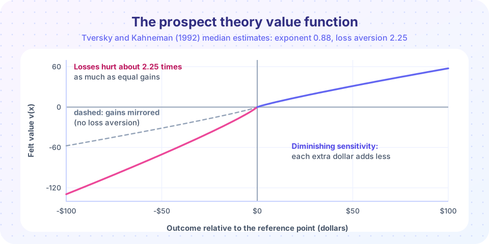
Both for gains and losses, the marginal impact shrinks as the amount grows. The curve is concave for gains and convex for losses, forming an S shape. A common formula, from Tversky and Kahneman (1992), is:
v(x) = x^0.88 for gains (x >= 0)
v(x) = -2.25 * (-x)^0.88 for losses (x < 0)
Here 0.88 is the curvature exponent (the median estimate in that study) and 2.25 is the loss-aversion coefficient, called lambda.
3. Loss aversion
The curve is steeper for losses than for gains. A loss of $100 is felt about 2.25 times as strongly as a gain of $100 in those estimates. This asymmetry is what makes the $110/$100 coin flip unattractive.
Worked example: the coin flip
Take the flip: 50% win $110, 50% lose $100. Using the formula (ignoring probability weighting for now):
v(110) = 110^0.88 = 62.6v(-100) = -2.25 * 100^0.88 = -2.25 * 57.5 = -129.4- Value of the gamble:
0.5 x 62.6 + 0.5 x (-129.4) = -33.4
The negative value means rejection. How large must the gain be for acceptance? Solve 0.5 x G^0.88 = 0.5 x 129.4, giving G^0.88 = 129.4, so G = 129.4^(1/0.88), about $250. People with these parameters need to win roughly $2.50 for every $1 they could lose. Because of diminishing sensitivity, the required ratio is a little above lambda, not exactly equal to it.
Note why this is not explained by risk aversion over wealth. For small stakes, concave utility over total wealth would make the gamble nearly risk neutral (recall Rabin's critique). Loss aversion over changes explains it neatly.
Evidence and everyday patterns
- Riskless choices. The endowment effect (next lessons) shows that giving up an object is valued more than acquiring it.
- Investing. Terrance Odean (1998) found that investors were more likely to sell stocks that had risen than ones that had fallen, relative to what they paid, consistent with the disposition effect. Taxes should push investors the other way, selling losers to claim tax benefits.
- Labor and prices. Workers resist pay cuts more than they welcome equivalent raises; consumers react more to price increases than to decreases.
How large is loss aversion, and is it universal?
The figure 2.25 is a median from a particular set of experiments. Estimates vary. A large meta-analysis of empirical estimates (Brown and colleagues, 2024) found an average near 2 across studies, with wide variation depending on the stakes, whether payments are real, and how the question is posed. Some researchers (for example Gal and Rucker, 2018) argue that evidence for loss aversion is weaker than often claimed and that other forces, such as status quo bias and attention, explain part of what is attributed to it. Others point out that for very small stakes there may be little or no loss aversion. A balanced view: loss aversion is a well-supported tendency in many settings, its strength varies, and "losses loom about twice as large as gains" is a useful rule of thumb, not a constant of nature.
Common misconceptions
- "Loss aversion means people refuse every gamble with a possible loss." It means a loss needs a larger gain to compensate; a big enough upside will be accepted.
- "The value function is the same as a utility function over wealth." It is defined over gains and losses from a reference point and has a kink at zero.
- "The number 2.25 is a law." It is a typical estimate from one study; other studies find different values.
Try it
First, compute with the value function and plot it. Change lam and alpha and re-run.
Press Run (or Ctrl + Enter) to see the result here.
Program input · what you'd type while the program runs
Type the answers before you press Run, one per line. Each time the program reads a line (with input()), it gets the next line from this box.
Second, an interactive model. Choose a gain and a loss size, a curvature and a loss-aversion level, and see whether this model would accept a 50/50 gamble. It is a demonstration of the formula, not a prediction for any particular person.
Check your understanding
Quick check · 5 questions
of 5 answered You scored / 5 · perfect!
-
1. What does the reference point do in prospect theory?
Outcomes are coded as changes relative to the reference point, usually the status quo. -
2. Which describes the shape of the value function?
Diminishing sensitivity gives the S shape; loss aversion makes the loss side steeper. -
3. With lambda = 2.25 and alpha = 0.88, would the model accept a 50/50 gamble to win $110 or lose $100?
The value is about -33, so the gamble is rejected despite its positive expected dollar value. -
4. The disposition effect is the tendency to
Realizing a gain feels good and realizing a loss feels bad, so investors hold losers and sell winners. -
5. What is the most accurate statement about the size of loss aversion?
Estimates differ by stakes and method, and some researchers dispute how general it is.
Summary
- Prospect theory values gains and losses relative to a reference point.
- The value function is concave for gains, convex for losses and steeper for losses (loss aversion).
- Typical estimates: exponent 0.88 and lambda 2.25; the average across studies is nearer 2 and varies with context.
- Loss aversion helps explain rejection of small favorable gambles, the disposition effect and resistance to price rises.
- Evidence is substantial but debated in its generality.
Next: Probability weighting
Track your progress
Create a free account to tick off lessons and pick up where you left off on any device.
of Behavioral Economics lessons completed