


















Lesson 41 of 47 · Markets, Finance and Policy Applications
Chapter 8 Review: Markets, Finance and Policy Applications
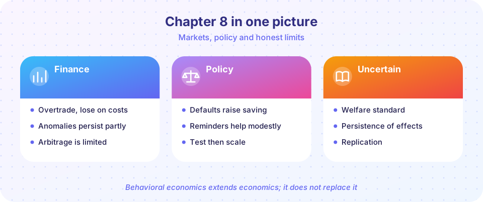
Review chapter 8 with a one-picture summary, a recap table of finance and policy findings, and a ten-question quiz on trading, loss aversion, megastudies and welfare.
Chapter 8 moved from laboratory choices to markets and public programs. In finance, households trade too much, sell winners too readily and look at their portfolios too often; at the market level, anomalies exist but weaken and are hard to exploit. In policy, defaults, reminders and clearer disclosure help at modest cost, megastudies show what typically works, and welfare questions and critiques keep the field honest. Use this page to consolidate.
What you will learn
- A single recap of the chapter's findings and numbers.
- How the disposition effect is measured.
- A self-test across the finance and policy lessons.
Recap table
| Topic | Key point |
|---|---|
| Overtrading | Most active households earned about 11.4 percent versus about 17.9 percent for the market (Barber and Odean) |
| Disposition effect | Gains realized more readily than losses (about 15 percent versus about 10 percent in Odean's data) |
| Myopic loss aversion | Frequent checking plus loss aversion makes stocks look risky; the gain-loss ratio rises with the horizon |
| Naive diversification | The 1/n rule makes the menu drive the allocation |
| Limits to arbitrage | Risk and funding constraints let mispricing persist |
| Anomalies | Many weaken after publication (McLean and Pontiff) |
| Pension defaults | The default rate shapes the pot for decades |
| Megastudies | Test many interventions at once; fewer than half beat the control in the gym study |
| Winner's curse | The best of many noisy estimates is overstated |
| Critiques | Welfare standard, heterogeneity, i-frame versus s-frame |
Try it
First, a toolkit with the chapter's calculations: the gain-loss ratio across horizons, the net return after trading costs and the pension pot.
Press Run (or Ctrl + Enter) to see the console output here.
No output.
Second, simulate how the disposition effect is measured. Twenty positions follow random price paths; the "neutral" investor sells winners and losers with the same daily probability, the "disposition" investor sells winners twice as often. The code computes the proportion of gains realized (PGR) and of losses realized (PLR). The ratio is the signature Odean looked for; the simulation uses assumed probabilities.
Press Run (or Ctrl + Enter) to see the result here.
Program input · what you'd type while the program runs
Type the answers before you press Run, one per line. Each time the program reads a line (with input()), it gets the next line from this box.
Check your understanding
Quick check · 10 questions
of 10 answered You scored / 10 · perfect!
-
1. Which investors earned the lowest net returns in Barber and Odean's study?
Trading costs and poor timing reduced the net returns of the most active households. -
2. A PGR/PLR ratio of about 1.5 in a dataset indicates:
Investors realize a larger share of their paper gains than of their paper losses. -
3. For the illustrative normal model, how does the gain-loss ratio change as the evaluation period lengthens?
Over longer horizons gains dominate losses in expectation, so even a very loss-averse person accepts. -
4. Why can mispricing persist despite arbitrage?
Shleifer and Vishny (1997) and De Long et al. (1990) describe the limits. -
5. Which finding supports caution about market anomalies?
McLean and Pontiff (2016) found sizable post-publication declines. -
6. Why use a megastudy?
Putting programs on equal footing shows what typically works and how large effects are. -
7. What is the winner's curse?
Selecting the top noisy estimate selects lucky draws. -
8. A worker saves 3 percent versus 8 percent for 40 years in the chapter's model. Roughly how do the pots compare?
311,000 versus 117,000, a ratio of about 2.7. -
9. What does the 1/n heuristic imply?
Splitting equally across funds makes the allocation depend on what funds are offered. -
10. What is the i-frame versus s-frame critique?
Chater and Loewenstein argue that individual framing can crowd out structural change.
Summary
- Households' mistakes are well documented; market-wide anomalies are real but fragile and hard to exploit.
- Myopic loss aversion links checking frequency to perceived risk.
- Policy designs help at low cost, and megastudies and retesting guard against exaggerated claims.
- Welfare standards, heterogeneity and systemic critiques define the limits of behavioral policy.
Track your progress
Create a free account to tick off lessons and pick up where you left off on any device.
of Behavioral Economics lessons completed