


















Lesson 24 of 47 · Time and Risk Preferences
Discounting and Impatience
Learn the discounted utility model, why constant discounting is time consistent, and how hyperbolic discounting explains impatience that changes with delay.
Would you rather have 100 today or 110 in a week? Many people take the 100. Would you rather have 100 in 52 weeks or 110 in 53 weeks? Many of the same people wait for the 110. The gap between the two offers is identical, one week for 10 extra, yet the answer changes. This lesson explains why that pattern matters, starting from the standard model of time preference and ending with the curve that fits behavior better.
What you will learn
- The discounted utility model and the meaning of the discount factor.
- Why exponential discounting is time consistent and what the common difference effect is.
- How hyperbolic discounting differs and where it can come from.
- Other regularities in measured discount rates, and why measuring them is hard.
Key terms
Discount factor D(t): the weight given to a benefit that arrives after delay t; D(0) = 1.
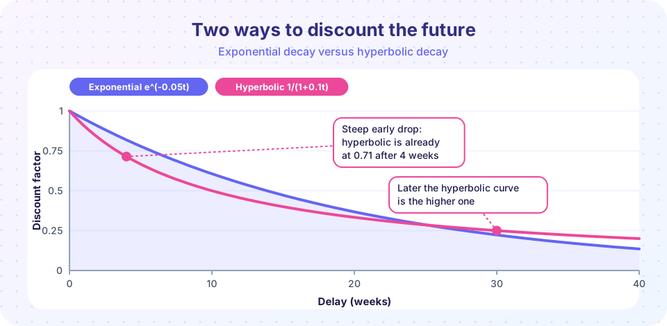
Exponential discounting: D(t) = δ^t, a constant percentage loss of value per period.
Hyperbolic discounting: D(t) = 1 / (1 + k·t), where the loss of value per period shrinks as the delay grows.
Common difference effect: choices between a smaller-sooner and a larger-later reward reverse when both are pushed equally into the future.
Implied discount rate: the yearly interest rate that would make an observed choice indifferent.
The discounted utility model
In 1937 Paul Samuelson proposed a compact way to describe choices over time. A person gets utility u(c_t) from consumption in each period t, and her total utility today is
U = u(c_0) + δ·u(c_1) + δ²·u(c_2) + ... = Σ δ^t · u(c_t)
The number δ (delta) is between 0 and 1. A value of 0.95 means that each extra period of waiting multiplies the weight by 0.95. The related interest-style rate is r = 1/δ − 1, so δ = 0.95 corresponds to r ≈ 5.3%. Samuelson was candid that this form was a convenient assumption, not a finding about psychology. Yet it became the default of economics because it has a powerful property.
Why constant discounting is time consistent
Under exponential discounting the relative weight on two future dates depends only on the gap between them. The weight on day 10 compared with day 11 is δ^10 : δ^11 = 1 : δ, whether you are standing on day 0 or day 9. So if you plan on day 0 to take the later reward, you will still want to on day 9. Robert Strotz showed in 1956 that without this property a person must treat her future selves as if they were different people who might not follow her plan.
Here is a worked example with δ = 0.9 per week. Compare 100 at week 0 with 110 at week 1: the first is worth 100, the second 0.9 × 110 = 99. The person takes 100 now. Now push both back 52 weeks: 0.9^52 × 100 versus 0.9^53 × 110. The ratio is the same, 110 × 0.9 = 99 against 100. She still takes the sooner reward. Exponential discounting never reverses.
What people actually do
Experiments find something different. Many participants choose the smaller sooner reward when it is available immediately, and choose the larger later reward when both are delayed. This is the common difference effect, and it is the signature of hyperbolic discounting.
The simplest hyperbolic form, introduced to psychology by George Ainslie and tested on animals by James Mazur, is:
D(t) = 1 / (1 + k·t)
Look at how fast the weight falls from one period to the next. The ratio D(t+1)/D(t) equals (1 + k·t) / (1 + k·t + k). At t = 0 with k = 0.1 it is 1/1.1 ≈ 0.91, a loss of about 9 percent per week. At t = 40 it is 5/5.1 ≈ 0.98, a loss of about 2 percent. The person is very impatient about the nearest wait and nearly patient about waits far away.
To see the reversal in numbers, take k = 0.1 per week. For 100 now versus 110 in a week: 100 versus 110/1.1 = 100, so the person is roughly indifferent now. Push both 10 weeks: 100/2 = 50 versus 110/2.1 = 52.4. The larger later reward wins, even though the choice looks the same.
Other regularities in measured discounting
Shane Frederick, George Loewenstein and Ted O'Donoghue reviewed the experimental literature in 2002 and found that the estimates of discount rates were remarkably scattered, from near zero to enormous, depending on the study. Several regularities recur:
- Delay effect: implied rates fall as delay grows (hyperbolic-like).
- Magnitude effect: small amounts are discounted more steeply than large ones.
- Sign effect: gains are discounted more steeply than losses of the same size.
- Sequence effects: people prefer improving sequences of outcomes to declining ones, which the simple model does not capture.
Their conclusion was cautious. The "discount rate" in the model bundles several psychological forces, such as impatience, expected change in circumstances, and uncertainty about whether the reward will arrive. Treating the bundle as one fixed parameter is a strong simplification.
Where hyperbolic curves may come from
One neat explanation comes from uncertainty. Suppose each period there is a chance h that the promised reward vanishes (the study ends, the promise is broken). A reward at delay t then survives with probability e^(−h·t), which is exponential. But if you do not know h, and your belief about it is itself spread out, averaging over possible h values gives a curve that falls fast at first and slowly later. Peter Sozou showed in 1998 that if your uncertainty about h is exponentially distributed with mean 1/a, the averaged weight is exactly hyperbolic, D(t) = 1 / (1 + t/a). Under this view, steep early drops reflect rational caution about a reward whose reliability you cannot judge. The second TryIt below checks this numerically.
Why measuring discount rates is hard
A choice between money now and money later is not a clean measure of patience. Three problems stand out.
- Money is not consumption. If a person can borrow or lend at a market rate, the choice between receiving money today or later may reflect that rate, not her patience. Experiments with small sums often find rates far above market interest rates.
- Curvature of utility. Discounting applies to utility, not money. If utility is concave, a person looks more impatient than she really is when you ignore the curvature. Steffen Andersen and coauthors (2008) estimated risk and time preferences together and found that discount rates came out lower once curvature was taken into account.
- Trust and transaction costs. A check that arrives in a month can feel uncertain or inconvenient even to a patient person.
The famous marshmallow studies by Walter Mischel and colleagues in the 1970s linked waiting at age four to later outcomes. A 2018 replication by Tyler Watts, Greg Duncan and Haonan Quan, with a larger and more diverse sample, found associations about half as large and mostly explained by family background and early cognitive skills. The lesson is that delay of gratification is real but sensitive to circumstances, including whether a child has reason to trust that a promised treat will arrive.
Common misconceptions
"A high discount rate means a person is irrational." A high rate can reflect need, risk or distrust. Irrationality in the narrow sense is inconsistency across time, not impatience.
"Hyperbolic discounting means people discount more overall." The defining feature is the shape: the rate declines with delay. A hyperbolic person can be patient on average and still reverse plans.
"The discount rate is one number you can look up." Estimates depend on method, stakes, sign, delay and the population, as Frederick and colleagues documented.
Try it
First, plot both curves and print the implied weekly rate for hyperbolic discounting at several delays.
Press Run (or Ctrl + Enter) to see the result here.
Program input · what you'd type while the program runs
Type the answers before you press Run, one per line. Each time the program reads a line (with input()), it gets the next line from this box.
Second, check Sozou's argument by simulation: average the survival curve e^(−h·t) over many random hazard rates and compare with the hyperbolic formula. This is a simulation that illustrates a mathematical result.
Press Run (or Ctrl + Enter) to see the result here.
Program input · what you'd type while the program runs
Type the answers before you press Run, one per line. Each time the program reads a line (with input()), it gets the next line from this box.
Third, a small tool for the common difference effect. It computes the value of a smaller-sooner and a larger-later reward under both models and tells you which one wins before and after the delay is added.
Press Run (or Ctrl + Enter) to see the console output here.
No output.
Check your understanding
Quick check · 5 questions
of 5 answered You scored / 5 · perfect!
-
1. In the model U = Σ δ^t u(c_t), what does a smaller δ mean?
A smaller δ shrinks the weight of future periods faster, so later benefits count for less. -
2. Why is exponential discounting time consistent?
Because the weight ratio of day t to day t+1 is always 1 to δ, a plan made today looks the same later. -
3. Hyperbolic D(t) = 1/(1 + 0.1 t). Roughly how much value is lost between week 0 and week 1?
D(1)/D(0) = 1/1.1, about 0.91, so about 9 percent is lost, much more than between weeks 40 and 41. -
4. Which finding is part of the common difference effect?
The reversal when both dates are pushed back is what exponential discounting rules out. -
5. Why might measured impatience in experiments be overstated?
Discounting applies to utility, not money, so joint estimation with risk preferences tends to lower estimated discount rates.
Summary
- Samuelson's discounted utility model weights period
tbyδ^t; it is time consistent because only the gap between dates matters. - Many people show the common difference effect, which fits hyperbolic discounting
1/(1 + k·t)with steep early drops. - Measured discount rates vary with delay, size and sign, and bundle impatience, uncertainty and utility curvature.
- Uncertainty about reliability can itself generate a hyperbolic curve, so steep early discounting is not automatically a mistake.
Track your progress
Create a free account to tick off lessons and pick up where you left off on any device.
of Behavioral Economics lessons completed