


















Lesson 26 of 47 · Time and Risk Preferences
Risk Attitudes in Practice
Learn how utility curvature gives risk aversion, what a certainty equivalent is, why Rabin's calibration argument challenges it, and how experiments measure risk.
Suppose someone offers a coin flip: heads you win 125, tails you lose 100. The average outcome is a gain of 12.50, yet plenty of sensible people say no. Is that a reasonable dislike of uncertainty, or evidence that our standard way of modeling risk is missing something? This lesson shows how economists represent risk attitudes, what a famous argument by Matthew Rabin says about small gambles, and how experimenters measure risk preferences with a simple list of choices.
What you will learn
- How the shape of the utility function encodes risk aversion, neutrality and risk seeking.
- How to compute a certainty equivalent and a risk premium.
- Why Rabin's calibration argument says curvature alone cannot explain small-stakes aversion.
- How the Holt-Laury price list measures risk attitudes, and why one number is not enough.
Key terms
Expected utility: the probability-weighted average of the utility of each outcome.
Certainty equivalent (CE): the sure amount that gives the same utility as a gamble.
Risk premium: expected value minus certainty equivalent; what a person gives up to avoid risk.
CRRA utility: u(x) = x^(1−ρ) / (1−ρ), with ln(x) for ρ = 1; ρ is the coefficient of relative risk aversion.
Multiple price list: a table of paired choices in which the odds change row by row.
Utility curvature and risk attitude
In expected utility theory, introduced by John von Neumann and Oskar Morgenstern, a person evaluates a gamble by the average utility of its outcomes:
EU = p1·u(x1) + p2·u(x2) + ...
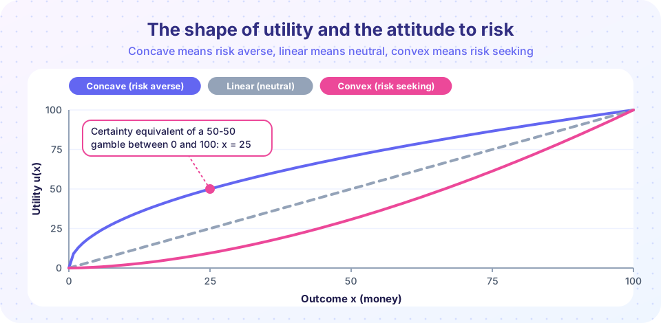
A concave u (it bends downward, like a square root) means each extra unit of money adds less than the one before. Then the pain of losing 50 is larger than the pleasure of gaining 50, and the person prefers the sure average to the gamble. That is risk aversion. A straight-line u is risk neutral, and a convex u is risk seeking.
A worked certainty equivalent
Take u(x) = √x and a 50-50 gamble between 0 and 100. The expected value is 50, but
EU = 0.5 × √0 + 0.5 × √100 = 5
The sure amount with utility 5 is x = 25, because √25 = 5. So the certainty equivalent is 25 and the risk premium is 50 − 25 = 25. This person would swap the gamble for a sure 25. The figure above shows the same thing: the point on the concave curve at utility 50 (on its 0-100 scale) sits at x = 25.
With CRRA utility the amount of curvature is summarized by ρ. For a 50-50 gamble between 20 and 100 (expected value 60) the certainty equivalent falls as ρ rises: about 52 for ρ = 0.5, about 45 for ρ = 1 (log utility) and about 33 for ρ = 2. You can reproduce these numbers in the first TryIt.
Rabin's calibration puzzle
Expected utility has a simple explanation for any risk aversion: curve the utility function. Matthew Rabin showed in 2000 that this explanation breaks down for small gambles. Here is the logic. If a person is risk averse because of curvature over her wealth, then a small gamble looks nearly like a fair bet from her point of view, since a small change in wealth hardly changes the slope of u. To reject a small favorable gamble she must have a lot of curvature. But a lot of curvature at small scale means a huge amount of curvature at larger scale.
Rabin's best-known example: suppose a person turns down a 50-50 gamble to lose 100 or gain 125 at every level of wealth. Then, he proved, she must also turn down a 50-50 gamble to lose 600 or gain 36 billion. No one believes that. So rejecting small gambles cannot be about curvature of utility over final wealth.
You can see the flavor of this with CRRA at a single wealth level. At wealth 20,000, rejecting "lose 100 or win 125" requires ρ of about 40. With ρ that high, the third TryIt shows that no gain, however large, would make a bet "lose 1,000, win G" acceptable. Utility is bounded above, so the large gain adds almost nothing.
What is the alternative? Rabin, with Richard Thaler, argued for loss aversion: people evaluate gains and losses relative to a reference point, and a loss hurts more than an equal gain pleases. This belongs to prospect theory (covered earlier in the course) and it explains small-stakes aversion without absurd consequences for large stakes. Critics have debated the technical assumptions of the argument (for instance, whether rejection "at all wealth levels" is plausible), but the practical message is widely accepted: curvature alone is a weak account of how people treat small risks.
Measuring risk attitudes
Charles Holt and Susan Laury introduced a popular method in 2002, the multiple price list. Each row offers a choice between two gambles:
| Option | High payoff | Low payoff |
|---|---|---|
| A (safer) | 2.00 | 1.60 |
| B (riskier) | 3.85 | 0.10 |
The chance of the high payoff rises from 10% in row 1 to 100% in row 10. A risk-neutral person compares expected values: 1.6 + 0.4p for A against 0.1 + 3.75p for B. They are equal at p ≈ 0.45, so she picks A in rows 1-4 and B from row 5 on: four safe choices. A more risk-averse person switches later. Under CRRA, about 5 safe choices means mild risk aversion and about 8 safe choices means ρ near 1. Holt and Laury also found that scaling all payoffs up several-fold made people choose the safe option more often, a sign that the same person is more risk averse when more is at stake.
Why one number is not enough
Several lines of research suggest that risk attitudes are not a single stable trait.
- Domains. A person may take physical risks but avoid financial ones; psychologists such as Elke Weber and colleagues measured domain-specific risk taking and perceived risk.
- Measures. Renato Frey and coauthors (2017) compared many behavioral tasks and self-reports in the same people. Behavioral measures correlated only weakly with each other, while self-reported risk taking showed a more coherent pattern.
- Noise. In price-list experiments a notable minority switch back and forth between A and B, which no single utility function can produce.
- Uncertainty types. Daniel Ellsberg showed in 1961 that people dislike ambiguity (unknown probabilities) over and above risk (known probabilities).
For policy this means that "the risk aversion parameter" in a model is a modeling choice. Where it matters, such as in insurance, retirement or financial advice, it is wise to measure it in the relevant context.
Common misconceptions
"Risk aversion means the person never takes gambles." A risk-averse person accepts any gamble whose certainty equivalent exceeds its price. Insurance and lotteries can be explained by different curvature and by probability weighting.
"A single number summarizes how risk averse someone is." Estimates vary by domain, by method and by stakes.
"Rabin proved that expected utility is false." He showed that explaining small-stakes risk aversion through curvature over wealth has absurd implications. Other versions of expected utility (for example with narrow framing) and other theories remain in use.
Try it
First, compute certainty equivalents for different degrees of curvature and plot them. This is a calculator for the CRRA formula, not a measurement of anyone's preferences.
Press Run (or Ctrl + Enter) to see the result here.
Program input · what you'd type while the program runs
Type the answers before you press Run, one per line. Each time the program reads a line (with input()), it gets the next line from this box.
Second, try a Holt-Laury style price list. Choose A or B in each row, then see how many safe choices you made. This is a demonstration of the format, not a test of your personality, and one session says little about your real risk preferences.
Third, map curvature to price-list behavior and then reproduce the Rabin-style calculation from the lesson. These are model calculations; the printed values come from the code.
Press Run (or Ctrl + Enter) to see the result here.
Program input · what you'd type while the program runs
Type the answers before you press Run, one per line. Each time the program reads a line (with input()), it gets the next line from this box.
Check your understanding
Quick check · 5 questions
of 5 answered You scored / 5 · perfect!
-
1. A person with u(x) = √x faces a 50-50 gamble between 0 and 100. What is her certainty equivalent?
EU = 0.5 × 0 + 0.5 × 10 = 5, and √25 = 5, so the certainty equivalent is 25. -
2. What does a concave utility function imply?
Diminishing marginal utility makes the sure average more valuable than a gamble with the same expected value. -
3. What is Rabin's main point about small gambles?
Enough curvature to reject a small favorable bet at every wealth level would make her reject enormously favorable large bets. -
4. In the Holt-Laury list, how many safe choices does a risk-neutral person make?
Expected values are equal at a high-payoff chance of about 45 percent, so she picks A in rows 1 to 4 and B afterward. -
5. Which finding suggests that risk attitude is not a single stable trait?
Studies such as Frey and coauthors (2017) find low agreement among behavioral tasks.
Summary
- In expected utility, concave utility means risk aversion; the certainty equivalent is the sure amount worth the same as a gamble.
- Rabin showed that curvature alone cannot explain why people reject small favorable bets without implying absurd choices for large ones; loss aversion offers an alternative.
- The Holt-Laury list measures risk attitude by where a person switches from the safe to the risky option, with four safe choices for a risk-neutral person.
- Risk attitudes vary with domain, stakes and measurement method, so treat any single estimate with care.
Next: Chapter 5 review
Track your progress
Create a free account to tick off lessons and pick up where you left off on any device.
of Behavioral Economics lessons completed