


















Lesson 39 of 47 · Markets, Finance and Policy Applications
Behavioral Finance
Explore behavioral finance: overtrading, the disposition effect, myopic loss aversion, limits to arbitrage, momentum, bubbles and what the evidence says about markets.
If you hold a share that has risen, do you sell it to lock in the gain? If you hold one that has fallen, do you hold on until it recovers? How often do you check your portfolio? Each of these small habits has been studied with data from hundreds of thousands of investors, and together they show how psychology reaches into financial markets. This lesson covers the main findings, from individual household mistakes to market-wide patterns, and is careful to separate what is solid from what is contested.
What you will learn
- What overconfidence and overtrading cost households.
- The disposition effect and why it looks like a mistake.
- Myopic loss aversion and the equity premium puzzle.
- Limits to arbitrage, momentum and bubbles, and how robust these findings are.
Key terms
Overconfidence: believing your judgment or information is better than it is.
Turnover: the share of a portfolio that is traded in a year.
Disposition effect: the tendency to sell assets that have gained value and hold on to those that have lost value.
Myopic loss aversion: loss aversion combined with frequent evaluation of results.
Momentum: the tendency of recent winners to keep outperforming over months.
Households trade too much
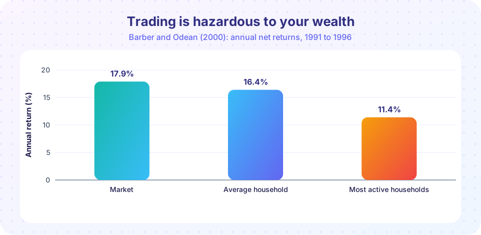
Brad Barber and Terrance Odean analyzed the trading records of 66,465 US households at a discount brokerage from 1991 to 1996. The market returned about 17.9 percent per year. The average household earned about 16.4 percent after costs. The households that traded most actively earned about 11.4 percent per year. Their stock picks were not much worse than the market before costs, but frequent trading generated costs such as commissions and bid-ask spreads that ate up the returns. Barber and Odean titled the paper "Trading Is Hazardous to Your Wealth", and in a follow-up, "Boys Will Be Boys" (2001), they showed that men traded about 45 percent more than women and earned lower net returns by roughly one percentage point per year, consistent with greater overconfidence.
Overconfidence is a plausible cause because people tend to overestimate the accuracy of their predictions and the value of their information. It is not the only one: investors may enjoy trading or treat it as entertainment. Barber and Odean (2008) also found that individual investors buy stocks that grab attention (those in the news or with unusually high trading volume), because choosing among thousands of stocks forces a search that attention cuts short.
The disposition effect
Hersh Shefrin and Meir Statman (1985) named the disposition effect: investors sell winners too early and hold losers too long. Terrance Odean (1998) tested it on the same kind of brokerage data. He compared the proportion of gains realized (sold) with the proportion of losses realized, and found about 15 percent versus about 10 percent: winning positions were sold more readily than losing ones.
Why call it a mistake? In many tax systems, realizing a loss gives a tax advantage, and selling winners triggers tax, so tax-wise the pattern should be reversed. Odean also found that the winners people sold went on to outperform the losers they kept, though only by a modest amount. Explanations include prospect theory (a gain is in the concave region, so a sure gain is attractive; a loss is in the convex region, where gambling to break even is attractive), regret avoidance (selling a loser makes the loss real) and mental accounting (treating each position as a separate account). The disposition effect has been documented in many countries and asset classes, although it is weaker among experienced investors.
Myopic loss aversion
Equities have historically returned more than bonds. Rajnish Mehra and Edward Prescott (1985) noted that the equity premium (about 6 percent per year in long US data) is far too large to be explained by standard risk aversion; it would require implausible levels of risk aversion. Shlomo Benartzi and Richard Thaler (1995) proposed myopic loss aversion: investors dislike losses roughly twice as much as they like equal gains, and they evaluate their portfolios often, so they perceive stocks as riskier than a long-horizon view suggests. With plausible loss aversion, they found that an evaluation period of about one year makes the observed premium consistent with investor behavior.
Here is the arithmetic. Suppose annual stock returns are normal with mean 7 percent and standard deviation 16 percent (an illustration). Over one year there is about a 33 percent chance of a loss. Over five years the chance is about 16 percent, over ten about 8 percent and over twenty under 3 percent. A loss-averse person who checks every year sees losses in a third of the checks and feels each one more than the gains. The ratio of expected gains to expected losses over the horizon (the gain-loss ratio) is about 3 at one year, but about 12 at five years and 37 at ten years. A person with loss aversion of 3.5 would turn down the one-year gamble but accept the five-year one. Experiments by Thaler, Tversky, Kahneman and Schwartz (1997) and by Uri Gneezy and Jan Potters (1997) found exactly this: participants who saw results more often took less risk.
Implications for practice include looking at retirement accounts less often, receiving reports that show long-term performance and automatic rebalancing that takes decisions out of the moment.
Naive diversification and fees
Shlomo Benartzi and Richard Thaler (2001) found that people often divide their retirement contributions roughly equally across the funds offered, the 1/n heuristic. If the menu has mostly stock funds, the portfolio is heavy in stocks; if mostly bond funds, it is heavy in bonds. The menu, not the person's risk tolerance, drives the allocation. In another experiment, James Choi, David Laibson and Brigitte Madrian (2010) gave participants index funds that held the same shares but charged different fees. Many did not choose the cheapest, even when fee information was in front of them.
Limits to arbitrage, momentum and bubbles
If mispricing exists, why do smart investors not remove it? Shleifer and Vishny (1997) show that arbitrage is risky. A mispriced asset can become more mispriced before it corrects, and arbitrageurs who manage other people's money may face withdrawals when losses mount. De Long, Shleifer, Summers and Waldmann (1990) add that traders who act on sentiment (noise traders) create risk that rational traders must bear.
Some market-level patterns have been interpreted this way:
- Long-term reversal. Werner De Bondt and Richard Thaler (1985) found that stocks that did badly over three to five years did better in the next period than past winners, which they read as overreaction.
- Momentum. Narasimhan Jegadeesh and Sheridan Titman (1993) found that stocks that did well over the past 3 to 12 months continued to do well for a few months.
- Excess volatility. Robert Shiller (1981) argued that stock prices fluctuate more than changes in dividends can justify.
- Bubbles in the laboratory. Vernon Smith, Gerry Suchanek and Arlington Williams (1988) created markets for an asset with a known fundamental value. Prices often rose far above value and then crashed. Bubbles shrink when the same traders gain experience (Dufwenberg, Lindqvist and Moore, 2005), but they appear robustly in many versions.
How robust are market anomalies?
Some of these patterns weaken once they become known. David McLean and Jeffrey Pontiff (2016) examined 97 published return predictors and found that returns were about a quarter lower outside the original sample and over half lower after publication. That suggests partly statistical flukes and partly traders learning to exploit them. Another reason for caution: patterns that look like irrational behavior may be compensation for risk, or reflect costs that are hard to measure. The reasonable conclusion is that individual-investor mistakes are well documented, while the claim that market prices are systematically wrong in ways that an ordinary investor can profit from is much harder to support.
Common misconceptions
"The disposition effect is just tax planning." Taxes would push investors to realize losses, the opposite of the observed pattern.
"Loss aversion means investors should avoid stocks." Myopic loss aversion is about how often you look; over long horizons the chance of a loss falls and the gain-loss ratio rises.
"Behavioral finance gives a recipe for beating the market." Most findings describe typical investor mistakes, not exploitable opportunities after costs.
Try it
First, an interactive view of myopic loss aversion. Move the slider to change how long the evaluation period is; the widget shows the chance of a loss and the gain-loss ratio for the normal-returns illustration (mean 7 percent, standard deviation 16 percent per year). A person with loss aversion λ accepts the stock gamble if λ is below the ratio.
Second, plot the gain-loss ratio across horizons with the same assumptions, and mark where a person with loss aversion 3.5 switches from rejecting to accepting.
Press Run (or Ctrl + Enter) to see the result here.
Program input · what you'd type while the program runs
Type the answers before you press Run, one per line. Each time the program reads a line (with input()), it gets the next line from this box.
Third, what overtrading costs. Suppose each investor picks stocks that earn the market's 8 percent gross return on average, and every round trip (buy and sell) costs 1.2 percent of the amount traded in commissions and spreads. The model shows net return against annual turnover. The cost is an assumption; real costs vary by investor and period.
Press Run (or Ctrl + Enter) to see the result here.
Program input · what you'd type while the program runs
Type the answers before you press Run, one per line. Each time the program reads a line (with input()), it gets the next line from this box.
Check your understanding
Quick check · 5 questions
of 5 answered You scored / 5 · perfect!
-
1. What did Barber and Odean find about the most active household traders?
Their net returns were around 11 percent per year versus about 18 percent for the market in the study period. -
2. What is the disposition effect?
Investors realize gains more readily than losses, the opposite of what tax rules reward. -
3. Myopic loss aversion combines:
Checking often exposes investors to many small losses, which loss aversion magnifies. -
4. Why is arbitrage limited, according to Shleifer and Vishny?
Risk and short horizons constrain professional arbitrage. -
5. What did McLean and Pontiff find about published return predictors?
About a quarter lower out-of-sample and over half lower after publication.
Summary
- Households tend to trade too much, and heavy turnover costs returns; overconfidence is one explanation.
- The disposition effect and naive diversification are robust household patterns.
- Myopic loss aversion explains why frequent checking makes stocks look risky; the gain-loss ratio grows with the horizon.
- Market-wide anomalies exist, but many weaken after publication, and limits to arbitrage explain why mispricing can persist.
Next: Behavioral policy
Track your progress
Create a free account to tick off lessons and pick up where you left off on any device.
of Behavioral Economics lessons completed