


















Lesson 7 of 47 · Rational Choice and Its Limits
Expected utility and Homo economicus
Learn the standard model of rational choice: preferences, utility, expected utility, risk aversion, certainty equivalents, and Rabin's critique with worked examples.
Every theory of choice starts with a question: what makes one option better than another for a particular person? The standard model answers with preferences and utility. When outcomes are uncertain it adds a rule for combining probabilities and utilities, called expected utility. This lesson builds the model step by step so that you can use it, and so that you can see exactly which of its pieces later lessons will question.
You will compute a certainty equivalent by hand and by code, and you will see why a curved utility function captures risk aversion.
What you will learn
- The two core assumptions about preferences: completeness and transitivity.
- How utility numbers represent preferences, and what they do not mean.
- How to compute expected value, expected utility, certainty equivalent and risk premium.
- Why a concave utility function means risk aversion, and what Rabin's critique says.
Key terms
Preference relation: a way of saying "A is at least as good as B" for pairs of options.
Completeness: for any two options, you prefer one or you are indifferent.
Transitivity: if you prefer A to B and B to C, you prefer A to C.
Expected value (EV): the probability-weighted average of the money outcomes.
Expected utility (EU): the probability-weighted average of the utilities of outcomes.
Certainty equivalent (CE): the sure amount that gives the same utility as the gamble.
Preferences and utility
Suppose you can compare any two options (completeness) and your comparisons never chase their tails (transitivity). Then your choices can be represented by a utility function, a number for each option such that you pick the option with the higher number. This is a representation, not a claim that anyone computes numbers in their head. "I choose coffee over tea" becomes u(coffee) > u(tea).
Note what is not assumed. Preferences can be strange, selfish or generous. The model only insists they be consistent. It also says nothing about the cardinal size of utility under certainty: only the ranking matters, until risk enters.
Choosing under risk: expected value is not enough
Offered a coin flip that pays $100 for heads and $0 for tails, what is the fair price? The expected value is 0.5 x 100 + 0.5 x 0 = 50. Many people, if asked, would take a sure $40 over this gamble, even though $40 is less than $50. So expected value cannot be the whole story: it ignores how people feel about risk.
In 1944 John von Neumann and Oskar Morgenstern showed that if preferences over gambles satisfy a handful of consistency axioms (completeness, transitivity, continuity and independence), then the person acts as if they maximize expected utility:
EU = p1 x u(x1) + p2 x u(x2) + ...
The utility function is bent by how much each extra dollar matters. The independence axiom, which says that mixing two gambles with a common third gamble does not reverse your preference, is the one that the Allais paradox (Lesson 2.4) attacks.
Risk aversion and the curved utility function
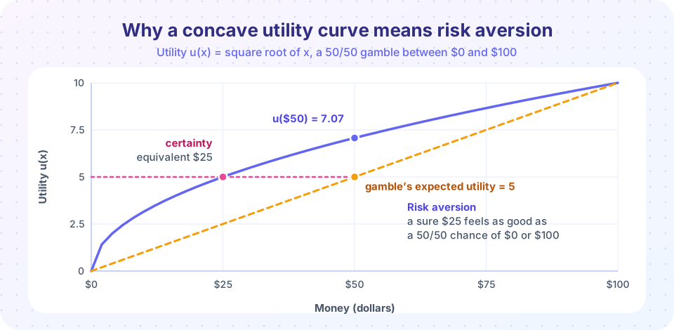
If every extra dollar adds less utility than the last, the utility curve is concave: it bends downward. Take the square-root function u(x) = sqrt(x). Then for the 50/50 gamble over $0 and $100:
EV = 50EU = 0.5 x sqrt(0) + 0.5 x sqrt(100) = 0.5 x 0 + 0.5 x 10 = 5- The certainty equivalent solves
sqrt(CE) = 5, soCE = 25. - The risk premium is
EV - CE = 50 - 25 = 25: this person would give up $25 of expected value to avoid the risk.
The picture above shows it: the straight chord from $0 to $100 lies below the curve. Concave utility means that a sure amount equal to the expected value beats the gamble, which is the definition of risk aversion. A straight-line utility gives risk neutrality (CE equals EV), and a convex one gives risk seeking.
A second worked example
Take a person with wealth of $1,000 and log utility u(w) = ln(w). Would they accept a 50/50 gamble that gains $100 or loses $50? The expected gain is +$25. Final wealth is $1,100 or $950.
EU(gamble) = 0.5 x ln(1100) + 0.5 x ln(950) = 0.5 x 7.0031 + 0.5 x 6.8565 = 6.9298
u(1000) = ln(1000) = 6.9078
Since 6.9298 is greater than 6.9078, they accept. Risk aversion is not the same as refusing every gamble: it says you demand a favorable enough deal.
Where does the theory strain?
Two criticisms matter for this course.
- Calibration. Matthew Rabin (2000) argued that if a person turns down modest-stakes gambles at all wealth levels, say a 50/50 bet to lose $100 or win $125, expected utility implies they would turn down absurdly attractive large bets, such as losing $600 against winning many billions. Since real people reject small bets but accept big ones, concavity of utility over wealth cannot be the explanation. Something else, such as loss aversion about changes (Chapter 4), is needed.
- Axioms. People systematically violate independence (Allais) and sometimes dislike unknown odds (Ellsberg). The next lessons take these up.
Common misconceptions
- "Utility is a measure of happiness." In the standard model it is only a representation of choice. It can be interpreted as happiness, but the theory does not require it.
- "Risk aversion means refusing all risk." It means preferring the sure expected value to the gamble; people still accept favorable gambles.
- "Rational means maximizing money." Rational agents maximize utility, and utility can depend on many things besides money.
Try it
First, compute certainty equivalents for the same gamble under different curvature. We use u(x) = x^a; for a = 1 the person is risk neutral and for a < 1 risk averse.
Press Run (or Ctrl + Enter) to see the result here.
Program input · what you'd type while the program runs
Type the answers before you press Run, one per line. Each time the program reads a line (with input()), it gets the next line from this box.
Second, an interactive picture. Move the slider to change the curvature of the utility function and watch the certainty equivalent move. This is a demonstration of the formula above, not a measurement of any person.
Check your understanding
Quick check · 5 questions
of 5 answered You scored / 5 · perfect!
-
1. A person has u(x) = sqrt(x). What is the certainty equivalent of a 50/50 gamble between $0 and $100?
EU = 0.5 x 0 + 0.5 x 10 = 5. Solving sqrt(CE) = 5 gives CE = 25. -
2. A concave utility function implies
Concavity means each extra dollar adds less utility, so a sure amount equal to the expected value beats the gamble. -
3. Which axiom does the Allais paradox challenge?
Allais showed that common preferences violate independence, the axiom that mixing with a common outcome should not reverse choices. -
4. What was Rabin's (2000) main point?
Rabin's calibration argument shows that concave utility over wealth cannot explain small-stakes risk aversion, which points to loss aversion and reference-dependence. -
5. Which is true of a risk-averse person who accepts a favorable gamble?
Risk aversion means preferring a sure EV to the gamble, not rejecting all gambles. A big enough edge overcomes it.
Summary
- The standard model rests on complete, transitive preferences represented by utility.
- Under risk, von Neumann and Morgenstern's axioms imply maximizing expected utility.
- Concave utility means risk aversion; the certainty equivalent is below the expected value, and the gap is the risk premium.
- Rabin's calibration argument and the Allais paradox show the theory's strain.
Track your progress
Create a free account to tick off lessons and pick up where you left off on any device.
of Behavioral Economics lessons completed