


















Lesson 42 of 46 · Projects and Practice
Project: a sensor signal chain from bridge to ADC
Design a strain-gauge signal chain: Wheatstone bridge, instrumentation amplifier gain, anti-aliasing filter, ADC range and resolution, with a numerical model of the whole chain.
Most real analog designs sit between the physical world and a digital system. A sensor produces a tiny voltage, an amplifier makes it usable, a filter removes what you do not want, and an analog-to-digital converter (ADC) turns it into numbers. Getting the levels right at every stage is the whole job: too small and the ADC sees nothing but noise; too large and the signal clips.
In this project you will design that chain for a classic sensor, a strain gauge that measures how much a metal beam bends, and follow the signal from bridge to number. The same design thinking applies to temperature sensors, pressure sensors and load cells.
What you will learn
- Compute the output of a Wheatstone bridge and choose an amplifier gain.
- Place the signal in the ADC range, including a reference level.
- Design an anti-aliasing filter and see what happens without one.
- Estimate resolution and noise.
Key terms
Strain (ε): relative length change; 1000 µε (microstrain) is 0.1%.
Gauge factor (GF): the ratio of the relative resistance change to the strain, ΔR/R = GF · ε; about 2 for a metal-foil gauge.
Wheatstone bridge: four resistors in a diamond whose differential output is zero when balanced and tiny when one resistor changes.
Instrumentation amplifier: a difference amplifier with very high input resistance and high CMRR, usually with three op-amps.
Aliasing: a signal above half the sampling rate that appears as a false lower frequency after sampling.
Step 1: the sensor and bridge
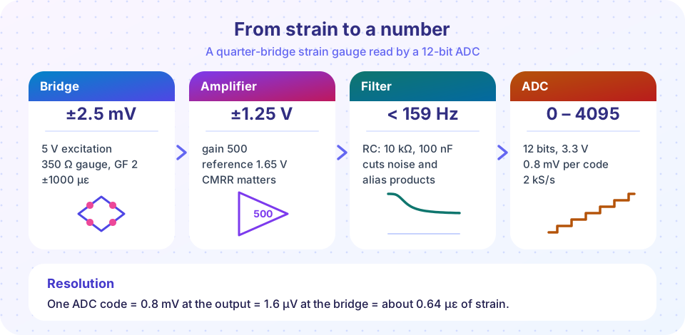
A 350 Ω gauge with GF = 2 stretched by ε = 1000 µε (0.1%) changes by ΔR/R = 2 × 0.001 = 0.2%, or 0.7 Ω. That is far too small to measure with a plain divider, so the gauge is placed in a bridge with three fixed 350 Ω resistors and excited by 5 V. For a quarter bridge (one active gauge) and small changes, the differential output is
Vbridge ≈ Vexc · (ΔR/R) / 4 = 5 V × 0.002 / 4 = 2.5 mV
So the full range of ±1000 µε produces ±2.5 mV, with a sensitivity of 2.5 µV per µε. Another benefit: the bridge output is differential and the common-mode level is half the excitation voltage (2.5 V), so the amplifier must reject a large common-mode voltage while amplifying microvolts. That is exactly what a difference amplifier with good CMRR does.
Step 2: the instrumentation amplifier
A three-op-amp instrumentation amplifier has a first stage of two non-inverting amplifiers sharing a gain resistor Rg, and a second stage that is a difference amplifier:
G = (1 + 2R / Rg) · (R2 / R1)
With R = 50 kΩ, Rg = 200 Ω and a unity second stage, G = 1 + 100k / 200 = 501, about 500. The output range is then ±2.5 mV × 500 = ±1.25 V. The ADC accepts 0 to 3.3 V, so the amplifier's reference pin is set to 1.65 V (half the ADC range). The output swings between 0.4 V and 2.9 V: centred, with headroom on both sides.
Real instrumentation amplifier chips (such as the INA series) have the three op-amps and precision resistors on one die, with CMRR of 100 dB or more. Choose a chip whose input bias current and noise are low, and add small RC filters at the inputs for radio-frequency interference.
Step 3: the anti-aliasing filter
Suppose the ADC samples at 2 kS/s. The Nyquist limit is 1 kHz. Anything above 1 kHz reaches the ADC and folds back as a false lower frequency. A 1.75 kHz interference signal, for instance, appears at 2000 - 1750 = 250 Hz. Once sampled, you cannot tell it from a real signal. The only cure is to filter before the ADC.
Our strain signals live below 100 Hz, so a first-order RC with fc = 159 Hz (10 kΩ, 100 nF) seems reasonable. But it attenuates 1.75 kHz only to 1 / √(1 + (1750/159)²) = 0.09, about -21 dB. A second-order Sallen-Key Butterworth at the same cutoff gives 1 / √(1 + 11⁴), roughly 0.008 (-42 dB). The demo below shows the difference. Practical designs often combine an analog filter with oversampling (sampling much faster, then filtering digitally).
Step 4: the ADC and resolution
A 12-bit ADC with a 3.3 V range has 4096 codes, so one code is 3.3 V / 4096 = 0.806 mV. Referred back to the bridge, divide by the gain: 0.806 mV / 500 = 1.6 µV, which corresponds to 1.6 µV / 2.5 µV per µε = 0.64 µε. So the system can resolve strain steps of about 0.64 µε. The theoretical thermal noise of the 350 Ω gauge is about 2.4 nV/√Hz, which over a 250 Hz noise bandwidth is only 38 nV rms, much smaller than one ADC code: the ADC, not the sensor, limits the resolution. To do better, increase the gain (reduces the range), use a higher-resolution ADC, or average many samples.
Common misconceptions
"The amplifier should just have as much gain as possible." Gain must fit the signal into the ADC range; excess gain clips the largest signals.
"A filter after the ADC can remove aliasing." Once the signal is sampled, an aliased component is indistinguishable from a real one. Filter before.
"Noise from the sensor decides everything." Often the amplifier or ADC noise dominates; compute the whole noise budget.
Try it
The first example simulates the entire chain numerically: strain, bridge, instrumentation amplifier with a hum pickup and a limited CMRR, the RC filter, sampling and 12-bit quantization. It reconstructs the strain from the codes. It is a model with a simple linear bridge and ideal amplifiers (apart from CMRR), not a measurement.
Press Run (or Ctrl + Enter) to see the result here.
Program input · what you'd type while the program runs
Type the answers before you press Run, one per line. Each time the program reads a line (with input()), it gets the next line from this box.
The second example demonstrates aliasing. A 50 Hz wanted signal and a 1.75 kHz interferer are sampled at 2 kS/s after no filter, a first-order filter and a second-order Butterworth filter, all with a 159 Hz cutoff. It reports the false 250 Hz component.
Press Run (or Ctrl + Enter) to see the result here.
Program input · what you'd type while the program runs
Type the answers before you press Run, one per line. Each time the program reads a line (with input()), it gets the next line from this box.
The third example is a level planner. Change the excitation, gauge factor, maximum strain and gain; it tells you whether the signal fits the ADC range with the 1.65 V reference.
Check your understanding
Quick check · 5 questions
of 5 answered You scored / 5 · perfect!
-
1. A quarter bridge with GF = 2.1 is excited with 10 V and strained by 500 µε. Approximately what is the bridge output?
Vout ≈ Vexc · GF · ε / 4 = 10 × 2.1 × 0.0005 / 4 = 2.6 mV. -
2. Why is the instrumentation amplifier's reference set to 1.65 V?
The amplifier output is ±1.25 V around the reference; 1.65 V centres it in the ADC range. -
3. A signal at 1.8 kHz is sampled at 2 kS/s. At what frequency does it appear?
It aliases to |2000 - 1800| = 200 Hz. -
4. What is the size of one ADC code for a 12-bit converter with a 3.3 V range?
3.3 V / 4096 = 0.806 mV. -
5. Why must the anti-aliasing filter be placed before the ADC?
Aliasing happens at the sampling instant; only an analog filter ahead of it can prevent it.
Summary
- A quarter bridge gives
Vexc · GF · ε / 4: millivolts that need an instrumentation amplifier with high CMRR. - Choose the gain so the output swings within the ADC range around a mid-supply reference.
- Anti-alias with an analog filter before sampling; a higher-order filter or oversampling helps.
- Resolution is the ADC step divided by the total gain and sensor sensitivity.
Track your progress
Create a free account to tick off lessons and pick up where you left off on any device.
of Analog Electronics lessons completed