


















Lesson 14 of 46 · Bipolar Transistors
The BJT small-signal model: gm, r-pi and a first amplifier
Linearize the transistor around its Q point with the hybrid-pi model: compute gm, r-pi and ro, then find the gain and resistances of a common-emitter amplifier.
A transistor's behavior is nonlinear: the collector current depends exponentially on the base-emitter voltage. Nonlinear equations are hard to solve by hand, and they do not obey superposition. But there is a way around this. If the signal is small compared with the DC conditions, then over a tiny stretch the exponential curve looks like a straight line, and a straight line is easy. The recipe is: find the DC operating point first, then replace the transistor by a small-signal model whose element values depend on that operating point, and analyze the signal with ordinary linear circuit analysis.
This is the single most useful technique in analog design. You will use it for every amplifier from here on.
What you will learn
- Why small-signal analysis works and what "small" means for a BJT
- The parameters g_m, r_π, r_e and r_o and how to compute each from the DC current
- How to draw the hybrid-π model and use it
- How to find voltage gain, input resistance and output resistance of a common-emitter stage
- How big the signal can get before distortion becomes visible
Key terms
Small signal: a signal small enough that the device behaves linearly around its Q point.
Transconductance (g_m): g_m = ∂I_C/∂V_BE = I_C/V_T, in siemens. It turns an input voltage into an output current.
r_π: the small-signal resistance looking into the base, r_π = β/g_m.
r_e: the small-signal resistance looking into the emitter, about 1/g_m (V_T/I_E).
Hybrid-π model: the standard small-signal equivalent circuit of a BJT.
Linearizing around the Q point
The exact law is i_C = I_s·e^(v_BE/V_T). Write the base-emitter voltage as a DC part plus a small signal: v_BE = V_BE + v_be. Then
iC = Is·e^(VBE/VT) · e^(vbe/VT) = IC · e^(vbe/VT) ≈ IC · (1 + vbe/VT)
using e^x ≈ 1 + x for small x. So the collector current is the DC value I_C plus a small signal:
ic = (IC / VT) · vbe = gm · vbe gm = IC / VT
The slope of the I_C–V_BE curve at the Q point is the transconductance. At 1 mA, g_m = 1 mA/25.9 mV = 38.6 mS (38.6 milliamps per volt, or 25.9 Ω as a reciprocal). It is directly proportional to the collector current, which is a very useful property: you can set the gain by choosing the bias current.
The other parameters
The base current is I_B = I_C/β, so the small-signal base current is i_b = i_c/β = g_m·v_be/β. The input resistance at the base is therefore
rπ = vbe / ib = β / gm
At 1 mA and β = 100, r_π = 100/38.6 mS = 2.59 kΩ. A larger collector current means a smaller r_π.
Looking into the emitter instead, the current is i_e = i_c + i_b, so
re = vbe / ie = 1 / gm × (β/(β+1)) ≈ VT / IE
which is about 26 Ω at 1 mA. This "internal emitter resistance" is worth remembering: r_e ≈ 26 Ω / I_E(mA).
Finally the Early effect gives the output resistance r_o = V_A/I_C (for V_A = 100 V at 1 mA, 100 kΩ), a resistor between collector and emitter.
The hybrid-π model
Replace the transistor by this circuit between the three terminals:
- a resistor r_π from base to emitter,
- a current source g_m·v_be from collector to emitter (controlled by the voltage across r_π),
- a resistor r_o from collector to emitter.
To use it, DC voltage sources (the supply) are replaced by grounds, because they do not change, and large capacitors are replaced by short circuits at the signal frequency. What remains is a simple linear circuit.
A common-emitter amplifier
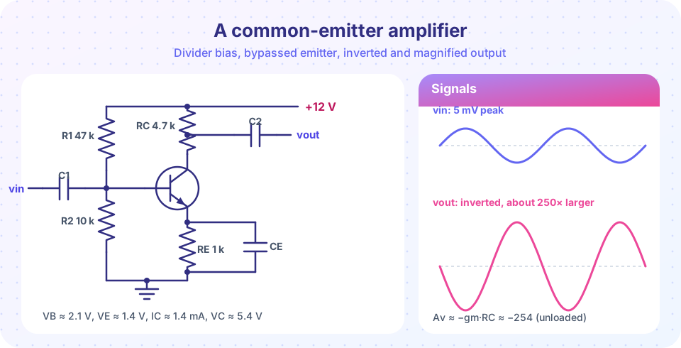
The circuit in the figure uses R₁ = 47 kΩ and R₂ = 10 kΩ to set the base voltage, R_E = 1 kΩ for stable bias, a bypass capacitor C_E to short R_E for signals, and coupling capacitors C₁ and C₂ to pass signals but block DC.
DC bias (estimate)
The divider sets V_B ≈ 12 × 10/57 = 2.1 V (neglecting base current). Then V_E = V_B − 0.7 = 1.4 V and I_E = 1.4 V/1 kΩ = 1.4 mA, so I_C ≈ 1.4 mA and V_C = 12 − 1.4 mA × 4.7 kΩ = 5.4 V. The collector sits 4 V above the emitter, comfortably in the active region. (If you include the base current with β = 100 the exact solution is I_C ≈ 1.29 mA, about 8 % lower. The Python example computes it.)
Small-signal gain
With I_C = 1.4 mA: g_m = 1.4 mA/25.9 mV = 54.1 mS and r_π = 100/54.1 mS = 1.85 kΩ.
For signals, R_E is bypassed, V_CC is ground, and the output sees R_C (in parallel with any load and r_o). The output voltage is v_out = −g_m·v_be·R_C, so
Av = vout / vin = −gm · (RC ∥ RL ∥ ro)
Unloaded, with r_o ignored: A_v = −54.1 mS × 4.7 kΩ ≈ −254. The minus sign means the output is inverted: when the input goes up, the collector current rises, the drop across R_C increases, and the collector voltage falls. With a 10 kΩ load, R_C ∥ R_L = 3.2 kΩ and A_v ≈ −173. Including r_o (about 70 kΩ here) trims both by roughly 6 %, to −239 and −166, and using the exact bias current of 1.29 mA lowers them to −220 and −153; the Python example below prints all of these. The lesson: the gain is only as accurate as the bias current behind it.
Input and output resistance
- Input resistance: the divider resistors R₁ ∥ R₂ = 8.25 kΩ appear in parallel with r_π: R_in = 8.25 k ∥ 1.85 k = 1.51 kΩ.
- Output resistance: looking back into the collector, R_out ≈ R_C = 4.7 kΩ (r_o is much larger and is in parallel).
If the signal source has an output resistance of 1 kΩ, the divider formed with R_in keeps only 1.51/(1 + 1.51) = 60 % of the signal at the base. The overall gain is about −254 × 0.60 ≈ −153 unloaded. This is the same loading effect you saw in chapter 1, applied to amplifier stages.
Without the bypass capacitor
If C_E is removed, R_E stays in the signal path. The emitter voltage then follows the base, and the gain drops to roughly
Av ≈ −RC / (re + RE) = −4.7 kΩ / (18.5 Ω + 1 kΩ) ≈ −4.6
Much lower, but it now depends almost only on resistor ratios, so it is stable against changes in β, temperature and the exact transistor. This trade of gain for stability, called negative feedback, is a central idea of chapters 5 and 6.
How small is small?
The linear approximation drops the quadratic term of the exponential. With x = v_be/V_T, the collector current is I_C·(1 + x + x²/2 + …), so the second-harmonic distortion is about x/4 = v_be/(4·V_T). For v_be = 1 mV that is about 1 %; for 5 mV about 5 %; for 10 mV nearly 10 %. A rule of thumb is that a common-emitter stage with no emitter resistance should have a base-emitter signal under a few millivolts, which is why the gain of such a stage is so large but its useful input range so small. Emitter resistance reduces distortion by cutting the signal that actually appears across the base-emitter junction.
Common misconceptions
"g_m is a fixed property of the transistor." g_m = I_C/V_T depends on the bias current. Double the current and g_m doubles.
"Small-signal analysis ignores DC." DC sets the model's values. You must do the DC analysis first, because g_m and r_π come from it.
"Voltage gain of −254 means the circuit amplifies any signal 254 times." Only small signals. A large input clips against the supply or distorts.
Try it
First, a complete numerical analysis of the amplifier: exact DC bias with finite β, the small-signal parameters, and the gains with and without load. Compare the exact values with the quick estimate from the text.
Press Run (or Ctrl + Enter) to see the result here.
Program input · what you'd type while the program runs
Type the answers before you press Run, one per line. Each time the program reads a line (with input()), it gets the next line from this box.
Second, a large-signal experiment. The program applies the exact exponential law to inputs of 1, 5 and 10 mV at the base and measures the second-harmonic distortion with a Fourier transform. The distortion grows in proportion to the input, as the x/4 rule predicts.
Press Run (or Ctrl + Enter) to see the result here.
Program input · what you'd type while the program runs
Type the answers before you press Run, one per line. Each time the program reads a line (with input()), it gets the next line from this box.
Check your understanding
Quick check · 5 questions
of 5 answered You scored / 5 · perfect!
-
1. A transistor is biased at I_C = 2 mA. With V_T = 25.9 mV, what is g_m?
g_m = I_C/V_T = 2 mA / 25.9 mV = 77.2 mS. -
2. With g_m = 40 mS and β = 100, what is r_π?
r_π = β/g_m = 100 / 0.04 = 2.5 kΩ. -
3. A common-emitter stage has g_m = 40 mS, R_C = 5 kΩ and a negligible load and r_o. What is the voltage gain?
A_v = −g_m·R_C = −0.04 × 5000 = −200. The minus sign means the output is inverted. -
4. What does removing the emitter bypass capacitor do?
R_E remains in the signal path, so A_v ≈ −R_C/(r_e + R_E): much lower but stable. -
5. Roughly what second-harmonic distortion results from a 5 mV peak signal across the base-emitter junction?
HD2 ≈ v_be/(4V_T) = 5 mV / 103.6 mV ≈ 4.8 %.
Summary
- Small-signal analysis linearizes the transistor around its DC Q point.
- g_m = I_C/V_T, r_π = β/g_m, r_e ≈ V_T/I_E, r_o = V_A/I_C. All depend on the bias current.
- The hybrid-π model has r_π (B–E), a current source g_m·v_be and r_o (C–E); supplies and large capacitors become grounds and shorts.
- A common-emitter stage has A_v = −g_m(R_C ∥ R_L ∥ r_o), moderate R_in = R₁ ∥ R₂ ∥ r_π and R_out ≈ R_C.
- Without a bypass capacitor the gain falls to about −R_C/(r_e + R_E) but becomes stable.
- Keep v_be to a few millivolts to limit distortion.
Next: Chapter 3 review
Track your progress
Create a free account to tick off lessons and pick up where you left off on any device.
of Analog Electronics lessons completed