


















Lesson 38 of 44 · Compressible Flow and Machinery
Pumps and turbines
How pumps and turbines exchange energy with a fluid: Euler's equation, head and power, pump curves, system curves, operating point, affinity laws and cavitation.
A pump is a machine that adds energy to a liquid; a turbine takes energy out. Both work by passing the fluid through a rotating set of blades. A centrifugal pump flings the liquid outward, a hydroelectric turbine is turned by falling water, and a fan or a jet engine compressor does the same job for gases.
The earlier lessons gave you the system side: how much head a pipeline demands. This lesson adds the machine side and shows how the two meet at one flow rate, the operating point.
What you will learn
- How Euler's turbomachine equation links blade speed to head.
- How to compute head, hydraulic power and efficiency.
- How to find an operating point from a pump curve and a system curve.
- What the affinity laws and cavitation tell a designer.
Key terms
Head (H): energy added per unit weight of fluid, in meters. For a pump, the head rise from inlet to outlet.
Efficiency (η): useful hydraulic power divided by shaft power, η = ρ g Q H / P_shaft for a pump.
Pump curve: the head a pump produces versus flow rate at a fixed speed.
Cavitation: formation and violent collapse of vapor bubbles where the local pressure falls to the liquid's vapor pressure.
Euler's turbomachine equation
Inside the impeller of a centrifugal pump, the blades turn the fluid and increase its angular momentum. Leonhard Euler's relation (1754) says the ideal energy transferred per unit mass is
W = U₂ V_θ2 − U₁ V_θ1
where U is the blade speed (ω r) and V_θ is the tangential (swirl) component of the absolute fluid velocity, at outlet (2) and inlet (1). Dividing by g gives the ideal head H_ideal = (U₂ V_θ2 − U₁ V_θ1)/g.
Example. An impeller of outer radius r₂ = 0.15 m turns at 1,450 rpm, so ω = 151.8 rad/s and U₂ = 22.8 m/s. If the fluid enters with no swirl and leaves with V_θ2 = 15 m/s, then H_ideal = 22.8 × 15 / 9.81 ≈ 35 m. Real pumps give less because of leakage, friction and recirculation, so the actual head and the efficiency come from tests.
The same equation, with the sign reversed, describes a turbine: the blades take angular momentum from the fluid.
Power and efficiency
- Hydraulic power delivered to the fluid by a pump:
P_h = ρ g Q H. - Shaft power needed:
P_shaft = P_h / η. Typical peak efficiencies are 60 to 85 percent for centrifugal pumps, higher for large ones. - Turbine: electrical power
P = η ρ g Q HwithHthe net head.
Example (hydropower). A turbine with Q = 10 m³/s under a net head H = 50 m and overall efficiency η = 0.90 gives P = 0.90 × 998 × 9.81 × 10 × 50 ≈ 4.4 MW.
Turbine types suit different heads and flows: Pelton wheels (impulse, jets hitting buckets) for high head and low flow, Francis (reaction) for medium head and flow, and Kaplan (axial propeller, adjustable blades) for low head and high flow.
Pump curve, system curve, operating point
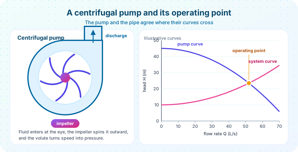
The pump curve falls as the flow increases. The system curve (Chapter 6) rises from the static lift as friction grows with Q². The pump runs where they cross, because there the head supplied equals the head required.
With the illustrative curves in the picture (Q in L/s, H in m), the pump curve is H = 45 − 0.008 Q² and the system curve is H = 10 + 0.005 Q². Setting them equal gives 35 = 0.013 Q², so Q ≈ 51.9 L/s and H ≈ 23.5 m. The hydraulic power is 998 × 9.81 × 0.0519 × 23.5 ≈ 11.9 kW.
If you throttle a valve, the system curve steepens and the operating point moves to a lower flow. If a filter clogs, the same thing happens. A well-chosen pump has its operating point close to its best efficiency point, where it works with the least internal loss.
Affinity laws
For geometrically similar pumps (or the same pump at different speeds), dimensional analysis (Chapter 5) gives constant flow, head and power coefficients. With speed N and impeller diameter D:
| Quantity | Scaling |
|---|---|
Flow Q |
N D³ |
Head H |
N² D² |
Power P |
ρ N³ D⁵ |
Raising the speed from 1,450 to 1,750 rpm (a factor 1.207) multiplies the flow by 1.207, the head by 1.457 and the power by 1.758. Power rises with the cube of speed, so a small drop in speed saves a lot of energy; that is why variable-speed drives are used on pumps and fans.
Cavitation and NPSH
On the inlet side of a pump, the pressure is lowest. If it falls to the vapor pressure of the liquid, bubbles form, then collapse violently when they reach higher pressure, causing noise, vibration and pitting damage. To avoid this, the net positive suction head available, NPSH_a = (p_in − p_v)/(ρ g) + V²/(2g), must exceed the NPSH_r required by the pump (from the manufacturer). Practical rules: keep suction pipes short and wide, place the pump low relative to the tank, and avoid hot liquids near boiling.
Common misconceptions
"A bigger pump always delivers more flow." The operating point depends on the system. A pump into a high-resistance system gives less flow than into a low-resistance one.
"Efficiency is constant." It varies with flow and peaks near the design point; running far from it wastes energy and can damage the pump.
"Pumps lift liquid by sucking." Atmospheric pressure pushes liquid into the inlet. Suction lift is limited, in the best case to about 10 m of water at sea level, and in practice much less.
Try it
First, find the operating point from the pump and system curves and plot it. Change the coefficients to see how the pump meets a different system.
Press Run (or Ctrl + Enter) to see the result here.
Program input · what you'd type while the program runs
Type the answers before you press Run, one per line. Each time the program reads a line (with input()), it gets the next line from this box.
Second, apply the affinity laws. The pump is run at three speeds against the same system, and the operating point slides along the system curve.
Press Run (or Ctrl + Enter) to see the result here.
Program input · what you'd type while the program runs
Type the answers before you press Run, one per line. Each time the program reads a line (with input()), it gets the next line from this box.
Check your understanding
Quick check · 6 questions
of 6 answered You scored / 6 · perfect!
-
1. A pump moves 0.05 m^3/s of water against a head of 30 m. What is the hydraulic power? (rho = 998, g = 9.81)
P = rho g Q H = 998 x 9.81 x 0.05 x 30 = 14,686 W = 14.7 kW. -
2. The pump speed is reduced by 20 percent. By what factor does the power change (affinity laws)?
Power scales with N^3, so 0.8^3 = 0.512. -
3. Where does a pump operate?
At that flow the head the pump supplies equals the head the system demands. -
4. What is cavitation?
Low local pressure makes the liquid boil locally; the collapse of the bubbles causes noise and damage. -
5. Which turbine type is best for a very high head and small flow?
Pelton wheels use high-speed jets and are used at heads of hundreds of meters. -
6. A throttle valve in the discharge line is closed partly. What happens to the operating point?
The valve adds resistance, steepening the system curve; the intersection moves up the pump curve to a lower flow and higher head.
Summary
- Euler:
H_ideal = (U₂V_θ2 − U₁V_θ1)/g; real machines are less efficient. - Hydraulic power
ρ g Q H; shaft power divides byη; turbines giveη ρ g Q H. - Pumps run where the pump curve meets the system curve.
- Affinity laws:
Q ∝ N D³,H ∝ N² D²,P ∝ N³ D⁵. - Avoid cavitation by keeping
NPSH_aaboveNPSH_r.
Next: Chapter 8 review
Track your progress
Create a free account to tick off lessons and pick up where you left off on any device.
of Fluid Mechanics lessons completed