


















Lesson 37 of 47 · Vibrations
Chapter 7 review: vibrations
A one-picture summary and ten mixed questions on free, damped and forced vibration of one-degree-of-freedom systems, with a quick design calculator.
One equation, m ẍ + c ẋ + k x = F(t), gave you three kinds of behavior: a steady ring at ωn, a decay controlled by ζ, and a driven response controlled by the frequency ratio r. Before starting the applications chapter, check that you can move between them.
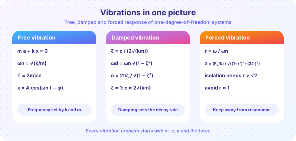
Recap table
| Concept | Formula | Remember |
|---|---|---|
| Natural frequency | ωn = √(k/m), T = 2π/ωn |
Independent of amplitude |
| Static deflection | δ_st = mg/k, ωn = √(g/δ_st) |
Gravity only shifts equilibrium |
| Damping ratio | ζ = c/(2√(km)) |
ζ < 1 oscillates |
| Damped frequency | ωd = ωn√(1 − ζ²) |
Slightly below ωn |
| Log decrement | δ = ln(x₁/x₂) = 2πζ/√(1 − ζ²) |
Measure ζ from a record |
| Forced amplitude | X = (F₀/k)/√((1−r²)²+(2ζr)²) |
Peak near r = 1 |
| Resonance | X = δ_st/(2ζ) at r = 1 |
Damping limits it |
A good routine
- Identify
m,c,k(orI,c_t,k_t) and the force. - Compute
ωn, thenζ. - If the question is about the free response, use
ωdand the envelope; if it is about a driving frequency, computer. - Check limits:
r → 0gives the static deflection,r → ∞gives a small, out-of-phase response.
Common mistakes
Mixing rad/s and Hz. Use ω in rad/s inside formulas; f = ω/2π.
Forgetting to compare c with c_cr. ζ, not c, tells you the damping level.
Using the free-vibration formula for a driven system. The steady response is at the driving frequency.
Using ζ in the formula as c/(2m ωn) with a wrong mass. Use the total moving mass.
Try it
A short design helper: given a machine mass, running speed and a target frequency ratio, it computes the mount stiffness and static deflection, and checks the response to a harmonic force.
Press Run (or Ctrl + Enter) to see the result here.
Program input · what you'd type while the program runs
Type the answers before you press Run, one per line. Each time the program reads a line (with input()), it gets the next line from this box.
The second tool is a general solver. It takes m, c, k, initial conditions and a force, integrates the response, and prints the main quantities.
Press Run (or Ctrl + Enter) to see the result here.
Program input · what you'd type while the program runs
Type the answers before you press Run, one per line. Each time the program reads a line (with input()), it gets the next line from this box.
Check your understanding
Quick check · 10 questions
of 10 answered You scored / 10 · perfect!
-
1. A 5 kg mass on a spring of 500 N/m has ωn of:
ωn = √(500/5) = 10 rad/s. -
2. A spring sags 25 mm under a mass. The natural frequency is about:
fn = 0.498/√0.025 = 3.15 Hz. -
3. ζ = 0.25 and ωn = 40 rad/s. What is ωd?
ωd = 40√(1 − 0.0625) = 38.7 rad/s. -
4. The magnification at resonance for ζ = 0.02 is about:
M = 1/(2ζ) = 1/0.04 = 25. -
5. Successive peaks of 6 mm and 3 mm give δ =
δ = ln 2 = 0.693. -
6. For r = 2 and light damping, the response is approximately:
M ≈ 1/(r² − 1) = 1/3 with phase near 180°. -
7. Which change lowers ωn?
ωn = √(k/m). -
8. A critically damped system has ζ =
By definition c = c_cr = 2√(km). -
9. A rotor unbalance force is 50 N at 100 rad/s. At 200 rad/s it is:
The force scales with ω², so doubling speed quadruples it: 200 N. -
10. Which statement about the steady forced response is true?
After the transient dies out, the system follows the force.
Summary
ωn,ζandrare the three numbers that describe a 1-DOF vibration.- Free:
x = x₀ cos ωn t + …; damped: envelopee^(−ζωn t); forced:Xfrom the magnification curve. - Avoid resonance by moving
rfar from 1; damp where you cannot. - Chapter 8 puts this to work in simulations and real mechanisms.
Track your progress
Create a free account to tick off lessons and pick up where you left off on any device.
of Engineering Dynamics lessons completed