


















Lesson 15 of 47 · Kinetics: Force and Acceleration
Drag and Variable Forces
Model linear and quadratic drag, find terminal velocity, and solve motion with speed-dependent forces using Euler and Runge-Kutta steps in Python.
So far every force was constant. Real forces are not. Air drag grows with speed, a spring pushes harder as it stretches, an engine's thrust changes with time. When the force depends on velocity, position or time, the acceleration is not constant and the simple v = v0 + a t fails. But ΣF = m a still holds at every instant. The price is that we must solve a differential equation, either by calculus (when we are lucky) or on a computer.
What you will learn
- The two common drag models and the idea of terminal velocity.
- How to solve
m dv/dt = m g − k vand its quadratic counterpart. - How Euler's method works and why a small time step matters.
- How to use a higher-order solver (
solve_ivp) for better accuracy.
Key terms
Linear drag: force proportional to speed, F = k v, typical for slow motion in thick fluids.
Quadratic drag: F = ½ ρ C_d A v² = k v², typical for objects in air at everyday speeds.
Terminal velocity: the steady speed at which drag balances weight (a = 0).
Time constant τ: the time scale of the approach to terminal velocity.
Euler's method: advance in small steps using v(t+Δt) ≈ v(t) + a Δt.
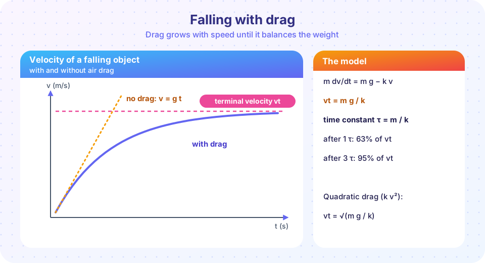
Linear drag
A particle falls with drag k v upward. Taking down as positive:
m dv/dt = m g − k v.
Separating variables or using an integrating factor gives v(t) = (m g / k) (1 − e^(−t/τ)) with τ = m/k. The terminal velocity is v_t = m g / k. After one time constant τ the speed is 63% of v_t; after 3 τ it is 95%.
Quadratic drag
For F = k v² (down positive): m dv/dt = m g − k v². Terminal velocity: v_t = √(m g / k). The solution is v(t) = v_t tanh(g t / v_t).
Worked example: a skydiver. Take m = 80 kg and ½ ρ C_d A = 0.42 kg/m (so ρ = 1.2 kg/m³ and C_d A = 0.7 m², a plausible belly-to-earth value for this model). Then
v_t = √(80 × 9.81 / 0.42) = 43.2 m/s(about 156 km/h);- 95% of
v_tis reached whentanh(x) = 0.95,x = 1.83, sot = 1.83 × 43.2 / 9.81 = 8.1 s.
Opening the parachute raises C_d A to maybe 25 m². Then k ≈ 15 kg/m and v_t = √(784.8/15) = 7.2 m/s: a survivable landing. The model's key message: terminal speed falls with the square root of the drag area.
Numerical solution
Most drag problems with extra features (wind, changing air density, thrust) have no closed form. The simplest numerical method is Euler:
a = (force at current state) / m
v = v + a * dt
x = x + v * dt
Smaller Δt means a smaller error, but the cost grows. Euler's error per step is proportional to Δt² and the global error to Δt, so halving the step halves the error. Better methods such as Runge-Kutta 4 (used by scipy.integrate.solve_ivp with method="RK45") are far more accurate for the same effort. Chapter 8 explores them further.
Common misconceptions
"Terminal velocity means no force acts." Drag and weight both act; they cancel, so the net force is zero.
"Heavier objects fall at the same terminal speed." v_t = √(m g/k) grows with mass: a steel ball reaches a higher terminal speed than a foam ball of equal size.
"A smaller time step always fixes everything." A tiny step reduces truncation error, but a wrong force law still gives wrong answers.
Try it
First, compare Euler's method with the exact quadratic-drag solution. Reduce dt and watch the gap shrink.
Press Run (or Ctrl + Enter) to see the result here.
Program input · what you'd type while the program runs
Type the answers before you press Run, one per line. Each time the program reads a line (with input()), it gets the next line from this box.
Second, use SciPy's adaptive solver and compare linear and quadratic drag with the same terminal velocity. The solver picks its own steps.
Press Run (or Ctrl + Enter) to see the result here.
Program input · what you'd type while the program runs
Type the answers before you press Run, one per line. Each time the program reads a line (with input()), it gets the next line from this box.
Check your understanding
Quick check · 5 questions
of 5 answered You scored / 5 · perfect!
-
1. At terminal velocity the net force on a falling object is
Drag balances weight, so the acceleration is zero. -
2. For quadratic drag F = k v², the terminal speed is
Set m g = k v² and solve. -
3. If you quadruple the drag coefficient k (quadratic drag), the terminal speed
v_t ∝ 1/√k, so a factor 4 in k halves the speed. -
4. With linear drag and τ = m/k, how fast is the object moving after t = 3 τ (starting at rest)?
1 − e^(−3) = 0.95. -
5. Euler's method with a smaller time step generally
The global error scales with Δt, at the price of more computation.
Summary
- Linear drag:
v_t = m g / k,v(t) = v_t (1 − e^(−t/τ)),τ = m/k. - Quadratic drag:
v_t = √(m g / k),v(t) = v_t tanh(g t/v_t). - Euler steps
v ← v + a Δt; use smaller steps or better solvers for accuracy. - Parachutes work because a larger drag area lowers terminal speed.
Next: Chapter 3 Review
Track your progress
Create a free account to tick off lessons and pick up where you left off on any device.
of Engineering Dynamics lessons completed