


















Lesson 38 of 47 · Applications and Simulation
Chapter 8 overview: simulating dynamic systems
Learn the simulation loop behind every dynamics program: state, forces, acceleration and time step, with a nonlinear spring and a bouncing ball as examples.
The chapters so far gave you closed-form answers: formulas for a falling ball, a rolling wheel, a damped oscillation. But most real systems do not have neat formulas. Add air drag that depends on speed squared, a spring that stiffens as it stretches, a ball that bounces, a motor with a control loop, and the equation of motion no longer has a textbook solution.
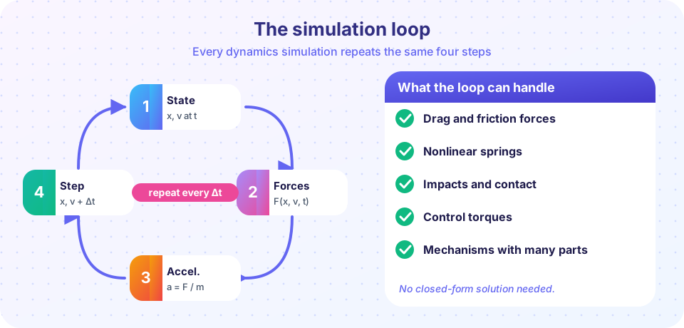
Simulation removes that barrier. You do not need to solve the equation: you only need to be able to compute the acceleration from the current state. Then you step forward a little in time, again and again. Every physics engine, every crash-test program and every robot controller runs a version of this loop.
What you will learn
- Describe the simulation loop and the role of the state vector.
- Turn a second-order equation into two first-order equations.
- Choose and check a time step.
- Use simple tests (energy, limiting cases) to trust a simulation.
Key terms
State: the minimal set of numbers that fixes the future of the system, e.g. position and velocity.
Time step Δt: the interval between updates.
Integrator: the rule that advances the state by one step.
Verification: checking the code against cases with known answers.
From Newton's law to a loop
Newton's law is second order: m ẍ = F(x, ẋ, t). A simulation uses first-order form. Define the state y = (x, v) and write
ẋ = v
v̇ = F(x, v, t) / m
Given the state at time t, you can compute the right-hand sides. The simplest update is
a  = F(x, v, t) / m
v  = v + a · Δt
x  = x + v · Δt      (this order is called semi-implicit Euler)
t  = t + Δt
For a rigid body in plane motion the state is (x, y, θ, ẋ, ẏ, θ̇), and the "forces" include moments divided by I. For a mechanism with n degrees of freedom the state has 2n numbers. The loop does not change: state, forces, acceleration, step.
Choosing the time step
A step that is too large gives inaccurate or even unstable results; one that is too small wastes time. A practical rule: Δt should be at least 20 to 50 times smaller than the shortest time scale in the system. For a vibration with period T, use Δt ≤ T/50. For a collision lasting 2 ms, you need steps of 0.05 ms or less. Halve the step and see whether the answer changes noticeably: if it does, the step was too large.
Trusting the result
Simulation errors are quiet: the program gives you a number either way. Build the habit of checking:
- Known case. Switch off the complicated part and compare with a formula (set the nonlinear term to zero and compare with
ωn = √(k/m)). - Energy. In a conservative system, total energy should stay constant. Drift means the step is too large or the method is wrong.
- Limits. Does the result behave sensibly for zero mass, zero damping, very large stiffness?
- Convergence. Does the answer settle as
Δtshrinks?
Write the state
Compute the push
Step and check
Common misconceptions
"Simulation replaces theory." You use theory to choose the model and to test the code.
"A smooth plot means a correct result." A wrong method can still give a pretty curve. Energy drift is the tell.
"Smaller steps always help." Past a point, rounding errors and run time dominate.
"The loop needs an exact solution." The loop needs only the acceleration as a function of the state.
Try it
First, watch a simulation run. This ball bounces on a floor with a coefficient of restitution e. Adjust e and the air drag and see how the bounces die away. The loop in the code is the one from this lesson.
Second, a problem without a closed-form answer. A mass on a "hardening" spring has force −k x − k₃ x³. The program simulates it for three amplitudes and estimates the period from zero crossings. For a linear spring all three would be equal.
Press Run (or Ctrl + Enter) to see the result here.
Program input · what you'd type while the program runs
Type the answers before you press Run, one per line. Each time the program reads a line (with input()), it gets the next line from this box.
Check your understanding
Quick check · 4 questions
of 4 answered You scored / 4 · perfect!
-
1. What is the state of a particle moving along a line?
Given position and velocity, plus the force law, the future follows. -
2. Why do simulations write m ẍ = F as two first-order equations?
Standard integrators advance the state vector using first derivatives. -
3. A vibration has a period of 0.05 s. A reasonable time step is about:
Δt ≤ T/50 = 0.001 s. -
4. Total energy in a conservative simulation slowly grows. What does it suggest?
Conservative systems keep energy constant, so drift signals numerical error.
Summary
- A simulation repeats: state, forces, acceleration, step.
- Write
m ẍ = Fasẋ = v,v̇ = F/mand advance byΔt. - Pick
Δtwell below the fastest time scale and test it by halving. - Verify with known cases, energy checks, limits and convergence.
Track your progress
Create a free account to tick off lessons and pick up where you left off on any device.
of Engineering Dynamics lessons completed