


















Lesson 11 of 43 · Survival Models and Life Tables
Chapter 3 overview: Survival models and life tables
See why actuaries model lifetimes as random, meet the survivor curve l(x), the future lifetime T(x) and the illustrative model used throughout this course.
Chapter 2 treated time as certain: a payment due in 10 years is made in 10 years. Insurance and pensions are different. A life annuity is paid only while the person lives, and a life insurance benefit is paid only when the person dies. Neither the number of payments nor the date of the benefit is known in advance. To value them we need a model of how long people live.
This chapter builds that model from the ground up: first as a curve showing how a group thins over time, then as a probability distribution, then as a table you can compute with. Chapter 4 will combine it with the interest tools you just learned to price benefits.
What you will learn
- Why lifetimes are modeled as a random variable and what that variable is.
- What the survivor curve
l(x)shows and how to read it. - How the illustrative Gompertz-Makeham model of this course is built.
- How the four lessons of the chapter fit together.
Key terms
Age at death X: a random variable, the age at which a newborn dies.
Future lifetime T(x): the number of years a person now aged x has still to live.
Survivor count l(x): the expected number alive at age x out of a starting group (the radix).
Radix l(0): the size of the starting group, often 100,000.
Mortality law: a formula for the force of mortality or survival function as a function of age.
Why a random lifetime?
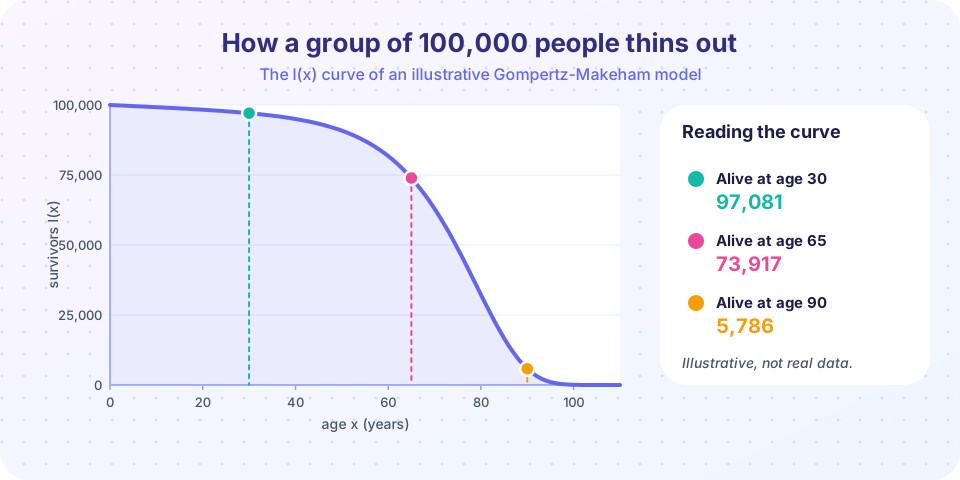
For a single person, the length of life is unknowable. For a population it is remarkably regular. Out of 100,000 newborns in our model, about 97,000 are alive at 30, about 74,000 at 65, about 5,800 at 90 and only a few dozen at 100. The curve on the picture is the average behavior of such a group. Individual lifetimes scatter around it, but the pooling of lesson 1.3 turns that scatter into predictable totals.
We therefore model the age at death as a continuous random variable X >= 0 with survival function S(x) = P(X > x). Then l(x) = l(0) S(x). The number who die between ages x and x + 1 is d(x) = l(x) - l(x + 1). A person already alive at age x has future lifetime T(x) = X - x, a random variable whose distribution is that of X conditioned on X > x. Everything in this chapter is a way of describing, computing and combining these ideas.
The model used in this course
To let you reproduce every number, the course uses a small mathematical model of mortality rather than a published table. Its force of mortality at age x is
mu(x) = A + B c^x with A = 0.0007, B = 0.00005, c = 1.1.
The constant A represents accident-type deaths that do not depend on age; the exponential term B c^x captures ageing, with mortality growing by 10% per year of age. This is the Gompertz-Makeham form, named after Benjamin Gompertz (1825) and William Makeham (1860), who first described how adult mortality rises roughly exponentially with age. The model is a good teaching device but a rough fit to real populations, with no infant-mortality spike and a faster rise at the highest ages than most real tables. Treat the numbers as illustrative.
Chapter 3 in four steps
From curve to money
What each lesson covers
- The survival function and force of mortality:
S(x),f(x),mu(x),t p xandt q x, the formula linking them. - Life tables:
l(x),d(x),q(x),p(x), life expectancy, using and building a table. - Select tables and fractional ages: what to do between birthdays, and why new policyholders die less often.
- Chapter 3 review: a one-page summary and mixed quiz.
Try it
First plot the survivor curve and the number of deaths at each age. The deaths curve (d(x)) peaks around age 79 in this model: the most common age at death, called the modal age.
Press Run (or Ctrl + Enter) to see the result here.
Program input · what you'd type while the program runs
Type the answers before you press Run, one per line. Each time the program reads a line (with input()), it gets the next line from this box.
Now simulate individual lives from the model. Each simulated person gets a random lifetime; the average of many is the life expectancy at birth. The simulation reproduces what the formulas predict, which is a good check that you understand the setup.
Press Run (or Ctrl + Enter) to see the result here.
Program input · what you'd type while the program runs
Type the answers before you press Run, one per line. Each time the program reads a line (with input()), it gets the next line from this box.
Common misconceptions
"Life expectancy at birth is how long most people live." It is the mean. In our model it is below the age by which most deaths occur, because early deaths pull the average down.
"A mortality law predicts one person's death." It describes proportions in a large group. For one person only the probability is meaningful.
"Real mortality follows the model exactly." Real mortality has infant deaths, accident humps at young adult ages, and changes over time and place. Models are approximations.
Check your understanding
Quick check · 4 questions
of 4 answered You scored / 4 · perfect!
-
1. If l(0) = 100,000 and l(65) = 73,917, how many of the 100,000 newborns are expected to die before 65?
100,000 - 73,917 = 26,083. -
2. What does T(x) denote?
T(x) = X - x, given that the person has survived to age x. -
3. In the Gompertz-Makeham force mu(x) = A + B c^x, what does the constant A represent?
A is the age-independent component, often thought of as accidental deaths; the exponential term models ageing. -
4. Which formula connects l(x) and the survival function S(x)?
The expected number alive at age x is the radix times the probability of surviving to x.
Summary
- A lifetime is a random variable
Xwith survival functionS(x) = P(X > x);l(x) = l(0) S(x). T(x)is the future lifetime of someone alive atx;d(x) = l(x) - l(x+1)counts deaths.- Our illustrative law has
mu(x) = 0.0007 + 0.00005 * 1.1^x: constant accidents plus exponential ageing. - The chapter covers survival functions, life tables, fractional ages and select tables.
Track your progress
Create a free account to tick off lessons and pick up where you left off on any device.
of Actuarial Mathematics lessons completed