


















Lesson 1 of 43 · Getting Started
Course map: Actuarial Mathematics
Start here: what actuarial mathematics is, who this course is for, the nine chapters, the prerequisites and a study plan with live examples.
Actuarial mathematics is the math of money that depends on uncertain events: whether a person lives to retirement, whether a house burns down, whether a pension fund can keep its promises for sixty years. Insurers, pension funds, regulators and consultants all hire actuaries to put numbers on those promises. This course teaches you the core toolkit step by step, with small invented companies and calculators you can run in your browser.
You do not need to be heading for an actuarial exam to enjoy it. If you like probability, compound interest or the idea of pricing the future, you will find a satisfying set of ideas here. If you are heading for professional exams (the Society of Actuaries, the Casualty Actuarial Society, the Institute and Faculty of Actuaries and others), the topics and notation follow the common international core, so the course works as a first pass before you pick up an exam manual.
What you will learn
- What actuaries do and why the same math appears in insurance, pensions and risk management.
- How the course is organized into nine chapters and which ones depend on which.
- Which prerequisites you need, and how to refresh them quickly.
- A study routine that fits worked examples, calculators and quizzes together.
Key terms
Actuary: a professional who uses probability, statistics and finance to measure and manage financial risk.
Premium: the price a policyholder pays for insurance cover.
Reserve: money an insurer sets aside today to pay claims that will fall due later.
Present value: what a future payment is worth today, after allowing for interest.
Mortality: the pattern of deaths in a population, described by probabilities of dying at each age.
The two ingredients: interest and uncertainty
Almost every calculation in this course combines two ingredients.
- The time value of money. A dollar next year is worth less than a dollar today because today's dollar can earn interest. Chapter 2 builds this idea carefully.
- Uncertainty about events. We do not know if a particular 40-year-old will live to 41, but we can describe the probability. Chapters 3 and 4 build mortality models and attach money to them.
An actuarial present value (APV) is simply a payment multiplied by the probability that it is made, multiplied by the discount factor for the waiting time. Everything else is organization and notation. Here is that idea in one picture of code. It prices "1 dollar paid in 10 years if the person is alive then", for a 40-year-old, using an illustrative mortality model we reuse throughout the course.
Press Run (or Ctrl + Enter) to see the result here.
Program input · what you'd type while the program runs
Type the answers before you press Run, one per line. Each time the program reads a line (with input()), it gets the next line from this box.
The result (about 0.587) is smaller than the plain discount factor because there is also a chance the person never collects. That "pure endowment" value is exactly one of the building blocks of chapter 4.
The nine chapters
Build the toolkit
Price and protect
Go further
Make it yours
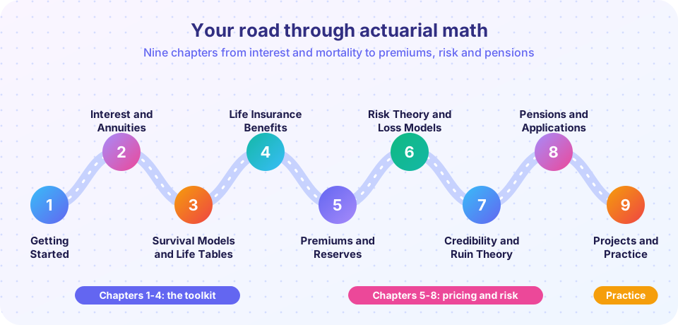
Chapters 1 to 4 are the toolkit and should be read in order. Chapter 5 uses all four. Chapters 6 and 7 can be read in either order once you know the basics of probability (chapter 1) and chapter 5 gives you the idea of a premium. Chapter 8 returns to the life models of chapters 3 and 4, applied to pensions. Chapter 9 combines everything.
Try the explorer below to see what each chapter feels like. It is a plain navigation demo, not part of the math.
Prerequisites and how to study
You need comfortable algebra (powers, logarithms, solving equations), the idea of a function and its graph, and basic calculus: derivatives and integrals appear from chapter 3 onward, mostly to connect rates and totals. If calculus is rusty, the integrals here are simple ones, and every formula is also given in a discrete form you can sum on a computer. Chapter 1 refreshes the probability you need.
A routine that works:
- Read the lesson once without stopping, looking at the picture first.
- Redo each worked example with a calculator or the code before reading the answer.
- Change the numbers in the runnable examples. Predict the effect, then check it.
- Take the quiz, and re-read any explanation that surprises you.
- At the end of each chapter, take the review quiz and try to explain the cheat-sheet picture from memory.
All mortality figures in this course come from a small mathematical model that we call illustrative. They are close enough to real life to teach with, but they are not real population data. Real actuaries use published tables or their own company data.
Common misconceptions
"Actuaries predict who will die." No. They describe the pattern for a large group, not any one person. The whole subject is built on the fact that groups are far more predictable than individuals.
"Insurance is just gambling." A gamble creates a new risk. Insurance pools an existing risk so its cost is shared and predictable.
Check your understanding
Quick check · 4 questions
of 4 answered You scored / 4 · perfect!
-
1. What two ingredients does almost every calculation in this course combine?
Interest turns future payments into present values, and probability tells us how likely each payment is. Together they give actuarial present values. -
2. An actuarial present value of 1 paid in 10 years if alive is smaller than v^10. Why?
The APV multiplies the discount factor v^10 by the probability of survival, which is below 1, so it must be smaller. -
3. Which chapter introduces life tables?
Chapter 3, Survival Models and Life Tables, builds the survival function and tables. -
4. Are the mortality numbers in this course real population data?
We use a small Gompertz-Makeham style model so that you can reproduce every number. Real work uses published or company tables.
Summary
- Actuarial math combines the time value of money with the probabilities of uncertain events.
- The course has nine chapters: toolkit (1 to 4), pricing and risk (5 to 8) and projects (9).
- Study with worked examples, runnable code and quizzes together.
- Mortality figures are illustrative; the methods are the real ones.
Next: What actuaries do
Track your progress
Create a free account to tick off lessons and pick up where you left off on any device.
of Actuarial Mathematics lessons completed