


















Lesson 27 of 43 · Risk Theory and Loss Models
Aggregate Claims and Compound Models
Combine claim counts and sizes into the total claim amount: mean, variance, the compound Poisson model, the Panjer recursion, simulation and premium loadings.
With a model for how many claims arrive and another for how big each is, you can build the quantity an insurer cares about most: the aggregate claim amount for a year. This is the number that decides whether the premiums collected will cover the claims, and how big a safety margin is needed.
The model is called the collective risk model because it treats the portfolio as one pool of claims rather than as individual policies. It is the standard tool for general insurance and for reinsurance pricing, and it is where the mathematics of this chapter pays off.
What you will learn
- State the mean and variance of a compound sum.
- Use the compound Poisson model and compute its distribution with the Panjer recursion.
- Simulate aggregate claims and compare with the normal approximation.
- Add a safety loading using the common premium principles.
Key terms
Compound distribution: the distribution of S = X₁ + … + X_N where N is itself random.
Compound Poisson: a compound distribution with Poisson N.
Panjer recursion: an exact method to compute the distribution of S when claims are discrete and N is in the (a, b, 0) family.
Safety loading θ: the proportion by which the premium exceeds the expected claims.
Coefficient of variation: the standard deviation divided by the mean.
Mean and variance of a random sum
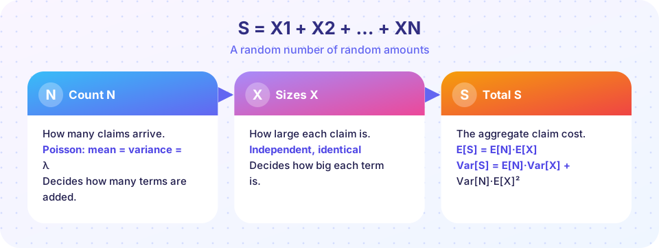
Let N be the number of claims and X₁, X₂, … the claim sizes, independent of each other and of N, all with the same distribution as X. Define S = X₁ + … + X_N, with S = 0 if N = 0. Conditioning on N gives two identities:
E[S]   = E[N] · E[X]
Var[S] = E[N] · Var[X] + Var[N] · (E[X])²
The variance has two sources: the randomness of claim sizes (first term) and the randomness of the number of claims (second term). For a compound Poisson, Var[N] = E[N] = λ, and the two terms combine into a neat expression:
Var[S] = λ · E[X²]
Worked example
Let λ = 2 claims a year and claim sizes 1, 2 or 3 (thousand currency units) with probabilities 0.5, 0.3 and 0.2.
E[X] = 0.5·1 + 0.3·2 + 0.2·3 = 1.7, soE[S] = 2 × 1.7 = 3.4.E[X²] = 0.5·1 + 0.3·4 + 0.2·9 = 3.5, soVar[S] = 2 × 3.5 = 7, standard deviation about2.65.
The exact distribution: Panjer recursion
Simulation gives approximate answers; for discrete claim sizes 1, 2, 3, … with probabilities f₁, f₂, … and f₀ = 0, the Panjer recursion gives the exact probabilities g_s = P(S = s). For compound Poisson:
g₀ = e^(−λ)
g_s = (λ / s) · Σ_{j=1..s} j · f_j · g_{s−j}      for s = 1, 2, 3, …
Check by hand with the example: g₀ = e^(−2) ≈ 0.1353; g₁ = 2 · 1 · 0.5 · g₀ ≈ 0.1353; g₂ = (2/2)(1 · 0.5 · g₁ + 2 · 0.3 · g₀) ≈ 0.1489. For negative binomial counts, use the general (a, b, 0) form g_s = Σ (a + b·j/s) f_j g_{s−j} / (1 − a f₀). Continuous claim sizes are first discretised into a grid.
Normal approximation and its limits
For a large portfolio, S is approximately normal with the mean and variance above, which gives quick answers such as P(S > E[S] + 2.33σ) ≈ 1%. But insurance totals are right-skewed; for small portfolios or heavy-tailed claims the normal approximation understates the upper tail. Always compare with simulation before trusting it.
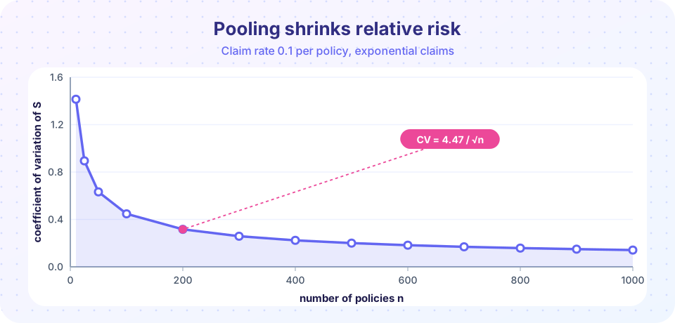
The picture shows why insurance is possible. When every policy has claim rate 0.1 and exponential claims, the coefficient of variation of S is 4.47/√n; a hundred times more policies makes the total ten times steadier relative to its mean.
Premium principles
An insurer charges more than the expected claims. Three classic rules for the premium H(S):
| Principle | Premium | Idea |
|---|---|---|
| Expected value | (1 + θ)·E[S] |
Proportional margin |
| Standard deviation | E[S] + α·σ_S |
Margin tied to risk |
| Variance | E[S] + α·Var[S] |
Margin tied to squared risk |
With the normal approximation, a loading θ gives probability Φ(θ · E[S] / σ_S) that premiums cover claims. For a fixed θ, this probability rises with the portfolio size because E[S]/σ_S grows like √n.
Try it
Press Run (or Ctrl + Enter) to see the result here.
Program input · what you'd type while the program runs
Type the answers before you press Run, one per line. Each time the program reads a line (with input()), it gets the next line from this box.
Press Run (or Ctrl + Enter) to see the result here.
Program input · what you'd type while the program runs
Type the answers before you press Run, one per line. Each time the program reads a line (with input()), it gets the next line from this box.
Common misconceptions
"Var[S] = E[N] × Var[X]." That ignores the variation in the number of claims. The full formula adds Var[N] · E[X]².
"A big portfolio has no risk." Independent claims average out, but any error in the assumptions (inflation, trend, a catastrophe affecting many policies) hits the whole portfolio at once.
"The normal approximation is always safe." For heavy-tailed claims or modest λ it understates the chance of a very large total.
Check your understanding
Quick check · 5 questions
of 5 answered You scored / 5 · perfect!
-
1. N has mean 4 and variance 4; X has mean 100 and variance 2500. What is Var[S]?
Var[S] = E[N]·Var[X] + Var[N]·E[X]² = 4·2500 + 4·10000 = 50,000. -
2. For a compound Poisson, Var[S] equals
Because Var[N] = λ, the two terms combine into λ·(Var[X] + E[X]²) = λ·E[X²]. -
3. In the Panjer example with λ = 2, the probability of no claims, g₀, is
S = 0 exactly when N = 0, which has Poisson probability e^(−λ). -
4. If the number of independent policies grows 100 times, the coefficient of variation of S falls by a factor of about
CV scales like 1 over the square root of the number of independent policies. -
5. A premium of E[S] + α·σ_S is called the
The margin is proportional to the standard deviation of the total claims.
Summary
E[S] = E[N]·E[X]andVar[S] = E[N]·Var[X] + Var[N]·E[X]²; for compound PoissonVar[S] = λ·E[X²].- The Panjer recursion computes the exact distribution of
Sfor discrete claim sizes and (a, b, 0) counts. - Pooling shrinks relative risk like
1/√n, which is the arithmetic behind insurance. - Premium principles turn spread into a loading: expected value, standard deviation or variance.
Track your progress
Create a free account to tick off lessons and pick up where you left off on any device.
of Actuarial Mathematics lessons completed