


















Lesson 16 of 43 · Life Insurance Benefits
Chapter 4 overview: Life insurance benefits
See how interest and survival combine: the present value random variable of a life benefit, its expected value, and a map of insurances, endowments and annuities.
Now the two halves of the course join. Chapter 2 told us how to value money paid at known times. Chapter 3 told us when a person dies, as a probability distribution. A life insurance policy pays a sum when the insured dies, which is a payment at a random time. Its value today is therefore a random variable, and its price is built from the mean of that variable.
The idea is simple, and the same idea covers every product in this chapter: write down the payment, the time it is made, and the event that triggers it. Discount it, and take the expected value.
What you will learn
- How to write the present value random variable
Zof a life benefit. - What the actuarial present value (APV) is and how to compute it.
- The three families of benefits: insurance, annuity, endowment.
- How the chapter's lessons fit together.
Key terms
Benefit: the amount paid under a policy, such as a sum assured on death.
Present value random variable Z: the discounted value at issue of the benefit actually paid; it depends on when the event occurs.
Actuarial present value (APV): E[Z], also called the expected present value or net single premium.
Curtate future lifetime K: the number of complete future years lived, K = floor(T).
Discrete vs continuous: whether benefits are paid at year ends or at the moment of death.
The present value random variable
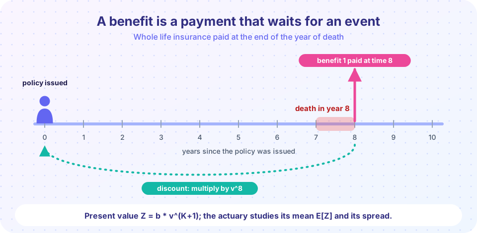
Take a whole life insurance of 1 on a person aged x, paid at the end of the year of death. Let K be the curtate future lifetime, the number of whole years completed before death. If the person dies in year K+1, the benefit is paid at time K+1 and its present value is
Z = v^(K+1).
The APV is E[Z] = sum over k >= 0 of v^(k+1) * P(K = k), where P(K = k) = k p x * q (x+k): survive k years, then die in the next. This is written A x. It is a mean of a payment made at different times with different discount factors, which is why neither the expected time of death nor the expected present value alone is enough: you must average v^(K+1), not compute v to the power of the average.
Worked example (three-year toy model). Suppose a person aged x can die in year 1, 2 or 3 with probabilities 0.1, 0.2 and 0.7, and i = 5%. Then E[Z] = 0.1 v + 0.2 v^2 + 0.7 v^3 = 0.095238 + 0.181406 + 0.604688 = 0.88133. The real-life version just has a longer list of years.
Three families of benefits
Pay when you die
Pay if you live
Mix them
- Insurances pay when the life ends (whole life) or if it ends within a period (term).
- Pure endowments pay a lump sum only if the person is alive at a stated date.
- Annuities pay a stream while the person lives.
- Endowment insurance combines a term insurance and a pure endowment, so a payment is made for sure, either at death or at maturity.
What each lesson covers
- Whole life and term insurance:
A x, term insurance, variance ofZ, recursions. - Endowments and pure endowments:
n E x, endowment insurance, and the payoff shapes. - Life annuities:
ä x, immediate and temporary annuities, and the linkA x = 1 - d ä x. - Chapter 4 review: formulas and a mixed quiz.
Try it
Simulate the present value of a whole life insurance of 1 for a 40-year-old with i = 5%. The simulation draws random lifetimes from the model, computes Z for each, and compares the sample mean with the exact APV obtained by summing v^(k+1) k|q.
Press Run (or Ctrl + Enter) to see the result here.
Program input · what you'd type while the program runs
Type the answers before you press Run, one per line. Each time the program reads a line (with input()), it gets the next line from this box.
The second example is an interactive reminder of how strongly the date of death matters to the value today. Slide the year of death and the interest rate.
Common misconceptions
"The APV is the discounted benefit at the expected year of death." The mean of v^(K+1) is not v^(E[K]+1). Because v^t is convex, the true mean is slightly larger.
"The insurer collects the APV at issue." The APV equals the single premium that exactly pays the expected benefit; most policies are paid by regular premiums with expenses added (chapter 5).
"Annuities and insurances are unrelated." They are linked by a simple identity you will meet in lesson 4.3.
Check your understanding
Quick check · 4 questions
of 4 answered You scored / 4 · perfect!
-
1. A person aged x can die in year 1 or year 2 with probabilities 0.4 and 0.6. With v = 0.9 and benefit 1 at the end of the year of death, what is E[Z]?
0.4 x 0.9 + 0.6 x 0.81 = 0.36 + 0.486 = 0.846. -
2. If K = 7 is the curtate future lifetime, in which year does death occur?
K counts completed years; death occurs in year K + 1 = 8, and the benefit is paid at time 8. -
3. Which product pays only if the person is alive at a stated future date?
A pure endowment pays a lump sum at maturity if the person has survived. -
4. What is the APV of a benefit?
APV = E[Z]; it is the net single premium for the benefit.
Summary
- Life benefits are payments at random times; their present value is a random variable
Z. - The APV is
E[Z]: sum of paymentxdiscount factorxprobability. - Whole life:
Z = v^(K+1), withP(K = k) = k p x * q (x+k). - Families: insurance (pay at death), pure endowment (pay if alive), annuity (stream while alive), endowment (mix).
Track your progress
Create a free account to tick off lessons and pick up where you left off on any device.
of Actuarial Mathematics lessons completed