


















Lesson 4 of 43 · Getting Started
Probability and expectation refresher
Refresh random variables, expectation, variance, conditional probability and the binomial, Poisson and exponential laws, with actuarial examples and live plots.
Every actuarial formula in this course is a statement about an expected value. The price of an insurance policy, the reserve for a pension, the present value of an annuity: each is an average of money over the possible futures, weighted by their probabilities. So this lesson refreshes exactly the probability you will use, with the notation actuaries prefer, and with examples taken from insurance rather than dice.
If you have studied probability recently, skim the headings and run the examples. If not, work through the worked examples slowly; they are short, and everything later depends on them.
What you will learn
- What a random variable, its distribution, mean and variance are.
- How to use indicator variables, the actuary's favorite trick.
- Conditional probability and conditional expectation, with a worked example.
- The binomial, Poisson, exponential and uniform distributions and when each appears.
Key terms
Random variable: a numerical outcome of a random event, such as the number of claims or the size of a claim.
Expected value E[X]: the probability-weighted average of the values of X.
Variance Var(X): E[(X - E[X])^2], a measure of spread; the square root is the standard deviation.
Conditional probability P(A | B): the probability of A given that B has happened.
Independent: events (or variables) that carry no information about each other.
Random variables, mean and variance
A discrete random variable X takes values x with probabilities P(X = x) that add up to 1. Its expectation is
E[X] = sum of x * P(X = x)
and its variance is Var(X) = E[X^2] - (E[X])^2.
Worked example. A policy pays 0 with probability 0.9, 1,000 with probability 0.09 and 5,000 with probability 0.01. Then E[X] = 0.09 x 1000 + 0.01 x 5000 = 90 + 50 = 140. And E[X^2] = 0.09 x 1,000,000 + 0.01 x 25,000,000 = 90,000 + 250,000 = 340,000, so Var(X) = 340,000 - 140^2 = 340,000 - 19,600 = 320,400 and the standard deviation is about 566. The rare large claim dominates the variance: 250,000 of the 340,000 second moment comes from the 1% event.
Three rules you will use constantly:
- Linearity:
E[aX + bY + c] = a E[X] + b E[Y] + c, always, even whenXandYare dependent. - Scaling:
Var(aX + b) = a^2 Var(X). - Independent sums: if
XandYare independent,Var(X + Y) = Var(X) + Var(Y).
For a continuous variable with density f(x), the sum becomes an integral: E[X] = integral of x f(x) dx. The survival model in chapter 3 uses exactly that.
The indicator trick
An indicator I_A equals 1 if event A happens and 0 otherwise. Its mean is P(A) and its variance is P(A)(1 - P(A)). Indicators are how actuaries write a payment that depends on an event: "pay 1,000 if the policyholder dies this year" is 1000 x I, with expected value 1000 q, where q is the death probability. Since expectation is linear, the expected total of many such payments is just the sum of the individual expectations, however they are related. This is why even a complicated book of policies can be priced one policy at a time.
Conditional probability and expectation
P(A | B) = P(A and B) / P(B). Conditional probability is how actuaries use information, such as age, smoking status or a good driving record.
Worked example. A motor insurer's customers are 30% young drivers and 70% experienced drivers. The probability of a claim in a year is 0.15 for young drivers and 0.05 for experienced drivers. What is the overall claim probability, and, given a claim, the probability the driver was young?
Overall: P(claim) = 0.3 x 0.15 + 0.7 x 0.05 = 0.045 + 0.035 = 0.08. This "law of total probability" is a weighted average over the groups. Given a claim: P(young | claim) = 0.045 / 0.08 = 0.5625. So young drivers are 30% of customers but about 56% of claims, which is why insurers price them separately.
The matching idea for averages is the law of total expectation: E[X] = E[ E[X | Y] ]. If you know the average claim in each group, the overall average is the weighted average of those averages. Chapter 6 uses it for compound claims.
The distributions you will meet
| Distribution | Typical use | Mean | Variance |
|---|---|---|---|
| Bernoulli(p) | one policy: claim or not | p | p(1-p) |
| Binomial(n, p) | claims among n independent policies | np | np(1-p) |
| Poisson(λ) | number of claims in a period (rare events) | λ | λ |
| Uniform(a, b) | a value equally likely anywhere in a range | (a+b)/2 | (b-a)²/12 |
| Exponential(λ) | waiting time to an event with constant rate | 1/λ | 1/λ² |
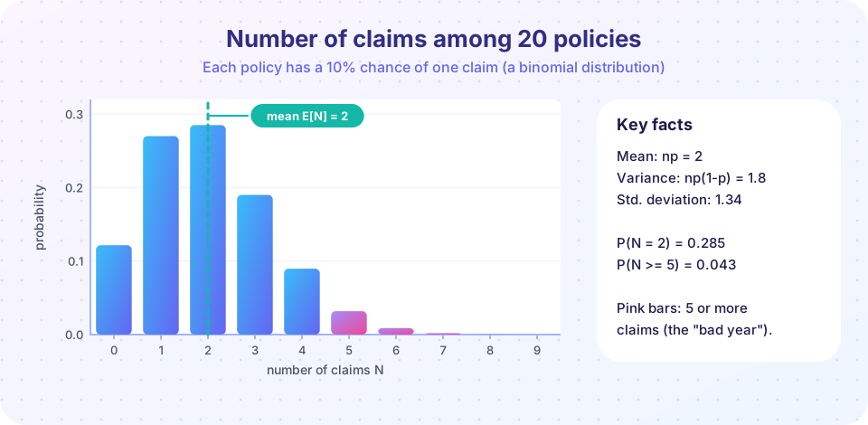
The binomial in the picture, with n = 20 and p = 0.1, has mean 2 and variance 1.8; the probability of exactly 2 claims is about 0.285, and the probability of 5 or more is about 0.043. The Poisson distribution is the limit of the binomial when n is large and p is small with np = λ fixed: it is the standard model for claim counts, and its mean equals its variance. The exponential distribution is the continuous cousin: if deaths occur at a constant rate λ, the time to death is exponential, with P(T > t) = exp(-λ t). A constant rate is the simplest "force of mortality" (chapter 3).
Try it
The first example computes moments for the discrete claim distribution above, then checks them with simulation. Compare the exact and simulated results.
Press Run (or Ctrl + Enter) to see the result here.
Program input · what you'd type while the program runs
Type the answers before you press Run, one per line. Each time the program reads a line (with input()), it gets the next line from this box.
The second example is an interactive visual: slide n and p and watch the binomial change, with its mean marked. It is a demonstration of the formulas above, not a model of any real portfolio.
Common misconceptions
"The expected value is the most likely value." The mean of the claim above is 140, but 140 is never an actual claim. The mean is an average over many policies, not a prediction for one.
"Var(X + Y) = Var(X) + Var(Y) always." Only when X and Y are independent (more precisely, uncorrelated). Linearity of the mean needs no such condition.
"A rare event can be ignored." The 1% event above supplies most of the variance. For pricing, rare large losses matter a great deal.
Check your understanding
Quick check · 5 questions
of 5 answered You scored / 5 · perfect!
-
1. A policy pays 2,000 with probability 0.05 and 0 otherwise. What is the expected payment?
E[X] = 0.05 x 2,000 = 100. -
2. What is Var(X) for a Bernoulli variable with p = 0.1 (X = 1 with probability 0.1)?
Var = p(1 - p) = 0.1 x 0.9 = 0.09. -
3. 30% of drivers are young with claim probability 0.15; 70% are experienced with claim probability 0.05. What is the overall claim probability?
0.3 x 0.15 + 0.7 x 0.05 = 0.045 + 0.035 = 0.08. -
4. Which distribution is the usual model for the number of claims in a period when claims are rare and independent?
The Poisson distribution is the limit of the binomial for many policies with small claim probability. Its mean equals its variance. -
5. If X and Y are dependent, which statement is always true?
Linearity of expectation holds with no independence condition. The other two need independence or zero covariance.
Summary
E[X]is the probability-weighted average;Var(X) = E[X^2] - (E[X])^2.- Expectation is linear, so portfolios can be priced policy by policy; variances add only for independent risks.
- Indicator variables write event-dependent payments as
payment x I, with meanpayment x probability. - Conditional probability and the law of total probability handle groups with different risks.
- Binomial and Poisson count claims; exponential models waiting times at a constant rate.
Next: Chapter 1 review
Track your progress
Create a free account to tick off lessons and pick up where you left off on any device.
of Actuarial Mathematics lessons completed