


















Lesson 26 of 43 · Risk Theory and Loss Models
Frequency and Severity Models
Learn the standard claim count and claim size distributions, how to read their tails, and how to fit them by matching moments, with worked examples and plots.
To model total claims you first need a model for the number of claims and a model for the size of one claim. These two choices are separate, and each has a short list of standard answers that actuaries have used for a century. The skill is knowing which answer to pick and what it implies about the risk.
This lesson introduces the counting distributions (Poisson and negative binomial), the severity distributions (exponential, lognormal and Pareto), and two tools for comparing them: the variance-to-mean ratio for counts and the mean excess function for sizes.
What you will learn
- Choose between Poisson and negative binomial counts using the variance-to-mean ratio.
- Compute means and variances of exponential, lognormal and Pareto claims.
- Explain what a heavy tail is and read it from a mean excess function.
- Fit a distribution by matching moments.
Key terms
Overdispersion: a variance larger than the mean in count data.
Survival function S(x): the probability that a claim exceeds x.
Heavy tail: a survival function that decays more slowly than any exponential.
Mean excess function e(d): the expected amount by which a claim exceeds d, given that it does.
Method of moments: choose parameters so that model moments equal sample moments.
Counting claims
The Poisson distribution
If claims arrive independently at a constant average rate, the number in a period is Poisson with mean λ:
P(N = k) = e^(−λ) λ^k / k! E[N] = Var[N] = λ
Equal mean and variance is the signature of the Poisson. It is the natural first model, and the building block of the compound Poisson in the next lesson.
The negative binomial
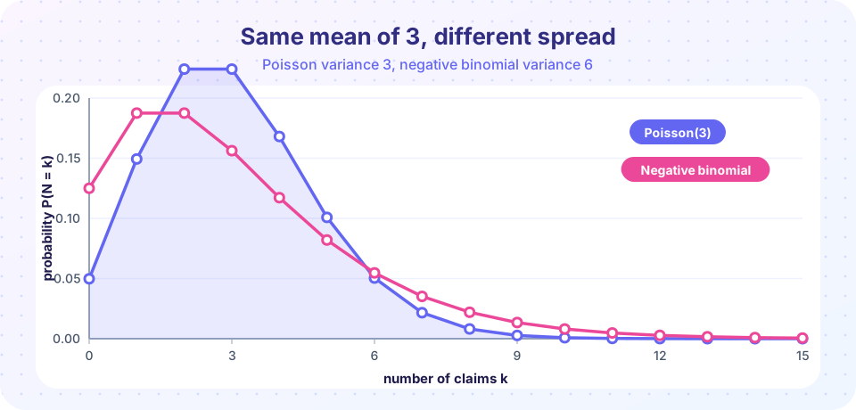
Real portfolios are rarely that tidy. Drivers differ: some are careful, some are not, and the portfolio's variance in counts is higher than the mean. One elegant explanation is that each policyholder has their own Poisson rate Λ, and the rates are spread according to a gamma distribution. Mixing a Poisson over a gamma gives the negative binomial with parameters r > 0 and β > 0:
E[N] = r·β Var[N] = r·β·(1 + β)
Here the variance exceeds the mean by the factor 1 + β, so a variance-to-mean ratio of 2 corresponds to β = 1. A negative binomial with the same mean as a Poisson has more mass at zero and in the upper tail.
The (a, b, 0) family
Both distributions satisfy a simple recursion in which each probability is a fixed function of the one before:
p(k) / p(k−1) = a + b / k for k = 1, 2, 3, …
| Distribution | a |
b |
|---|---|---|
| Poisson(λ) | 0 | λ |
| Negative binomial(r, β) | β/(1+β) | (r−1)·β/(1+β) |
| Binomial(m, q) | −q/(1−q) | (m+1)·q/(1−q) |
This family is what the Panjer recursion in the next lesson needs.
Sizing claims
Exponential, lognormal and Pareto
| Distribution | Survival function | Mean | Comment |
|---|---|---|---|
| Exponential(θ) | e^(−x/θ) |
θ |
Light tail, memoryless |
| Lognormal(μ, σ) | 1 − Φ((ln x − μ)/σ) |
e^(μ + σ²/2) |
Skewed, long but finite-moment tail |
| Pareto (Lomax)(α, θ) | (θ/(x+θ))^α |
θ/(α−1) for α > 1 |
Power-law tail |
For the lognormal, the variance is (e^(σ²) − 1)·e^(2μ + σ²). For the Pareto, the variance exists only if α > 2; for α ≤ 1 even the mean is infinite, which is a warning that such a line of business is hard to price.
What the mean excess function reveals
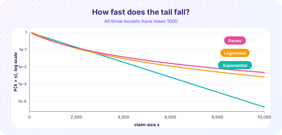
Given that a claim exceeds a threshold d, how much more do we expect? That is e(d) = E[X − d | X > d]. For the exponential it is a constant θ (memorylessness). For the Pareto it grows linearly, (θ + d)/(α − 1): if a claim is already large, it is likely to be much larger. For the lognormal it also grows. An increasing mean excess function is the quickest sign of a heavy tail and a hint that reinsurance may be needed.
Fitting by matching moments
Suppose a sample has mean m and second moment s₂ = E[X²] (or variance v = s₂ − m²).
- Lognormal:
σ² = ln(1 + v/m²)andμ = ln m − σ²/2. - Pareto:
α = 2(s₂ − m²)/(s₂ − 2m²)(requiress₂ > 2m²) andθ = m(α − 1). - Poisson:
λ =sample mean. If the sample variance is much larger, switch to the negative binomial withβ = (v/m) − 1andr = m/β.
Moment matching is quick and transparent; maximum likelihood is more efficient but needs numerical optimisation. Actuaries usually start with moments, then refine.
Try it
Press Run (or Ctrl + Enter) to see the result here.
Program input · what you'd type while the program runs
Type the answers before you press Run, one per line. Each time the program reads a line (with input()), it gets the next line from this box.
Press Run (or Ctrl + Enter) to see the result here.
Program input · what you'd type while the program runs
Type the answers before you press Run, one per line. Each time the program reads a line (with input()), it gets the next line from this box.
Press Run (or Ctrl + Enter) to see the result here.
Program input · what you'd type while the program runs
Type the answers before you press Run, one per line. Each time the program reads a line (with input()), it gets the next line from this box.
Common misconceptions
"Claim sizes are normally distributed." Claims are bounded below by zero and heavily right-skewed; the normal is a poor model except for totals of many claims.
"If the sample variance equals the mean, the data are Poisson." Equal first two moments are necessary, not sufficient; check the whole distribution, and think about whether policyholders really have the same rate.
"A Pareto with a finite mean is safe." If α is only slightly above 1 the mean exists but sample averages converge extremely slowly.
Check your understanding
Quick check · 5 questions
of 5 answered You scored / 5 · perfect!
-
1. A sample of claim counts has mean 2 and variance 5. Which model is more suitable?
The variance exceeds the mean (overdispersion), which a Poisson cannot produce but a negative binomial can. -
2. The mean excess function of the exponential distribution with mean θ is
The exponential is memoryless: given that a claim exceeds d, the excess has the same exponential law. -
3. A Pareto (Lomax) with α = 4 and θ = 3000 has mean
Mean = θ/(α − 1) = 3000/3 = 1000. -
4. For the negative binomial with r = 2 and β = 0.5, the variance of N is
Var = rβ(1 + β) = 2 × 0.5 × 1.5 = 1.5, which is larger than the mean rβ = 1. -
5. Matching moments for a lognormal gives σ² = ln(1 + v/m²). If the coefficient of variation squared v/m² is 0, then
Zero variance gives ln 1 = 0, so there is no spread in the log of the claim.
Summary
- Poisson counts have equal mean and variance; the negative binomial adds overdispersion and arises as a gamma mixture of Poissons.
- Exponential, lognormal and Pareto claims differ most in their tails; the mean excess function shows whether the tail is light or heavy.
- Method of moments gives quick parameter estimates: it is a starting point, not the final word.
Track your progress
Create a free account to tick off lessons and pick up where you left off on any device.
of Actuarial Mathematics lessons completed