


















Lesson 13 of 43 · Survival Models and Life Tables
Life tables
Learn to read, use and build life tables: survivors l(x), deaths d(x), probabilities q(x) and p(x), multi-year probabilities and life expectancy, with code.
A formula for mu(x) is elegant, but for day-to-day work actuaries prefer a table. A life table lists, for each age, how many of a starting group of newborns are expected to be alive, how many will die in the next year, and the resulting probabilities. All of the probabilities you need in chapter 4 come from simple ratios of table entries, with no calculus.
Real life tables are published by national statistics offices, by the actuarial societies and by insurers from their own experience. In this lesson you will learn how to read one, build one from a model, and extract probabilities and life expectancy from it. We use the illustrative model of this chapter; the steps are identical for a real table.
What you will learn
- What each column of a life table means and how the columns are linked.
- How to compute
t p x,t q xand deferred probabilities froml(x). - How to compute curtate and complete life expectancy from a table.
- The difference between period and cohort tables, and why tables date.
Key terms
Radix: the starting number l(0) or l(x0), often 100,000.
d(x): expected deaths between ages x and x + 1.
q(x), p(x): probabilities of dying and of surviving the year after age x.
Period table: based on the deaths of a single calendar period, applied as if everyone experienced that period's mortality.
Cohort table: follows people born in a given year through their actual (or projected) lives.
The columns
Given l(x), everything follows:
| Symbol | Meaning | Formula |
|---|---|---|
l(x) |
expected survivors to exact age x |
given |
d(x) |
deaths between x and x+1 |
l(x) - l(x+1) |
q(x) |
probability of dying within a year, age x |
d(x) / l(x) |
p(x) |
probability of surviving the year | l(x+1) / l(x) = 1 - q(x) |
t p x |
survive t years |
l(x+t) / l(x) |
t q x |
die within t years |
(l(x) - l(x+t)) / l(x) |
The deferred death probability (survive t years, then die within the next u) is (l(x+t) - l(x+t+u)) / l(x). It is written t|u q x in actuarial notation.
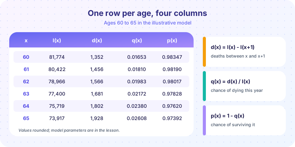
In the picture, l(60) = 81,774 and l(61) is slightly smaller, so about 1,350 die in the year: q(60) = 0.01653. Notice the denominator: all the probabilities for someone aged x divide by l(x), not by the radix. The table is a way to keep conditional probabilities in one place.
Worked example. Using l(60) = 81,774, l(65) = 73,917 and l(70) = 62,953:
5 p 60 = 73,917 / 81,774 = 0.9039: a 60-year-old has a 90.4% chance of reaching 65.5 q 60 = 1 - 0.9039 = 0.0961.- The probability a 60-year-old survives to 65 and then dies before 70 is
(73,917 - 62,953) / 81,774 = 10,964 / 81,774 = 0.1341.
Building a table from a model
If you have mu(x) or S(x), compute l(x) = l(0) S(x) at integer ages, then subtract. The code below builds the table used in this course and prints the same rows as in the picture, then reproduces the worked example.
Press Run (or Ctrl + Enter) to see the result here.
Program input · what you'd type while the program runs
Type the answers before you press Run, one per line. Each time the program reads a line (with input()), it gets the next line from this box.
Life expectancy from a table
The curtate expectation of life counts complete years lived: e_x = sum over k >= 1 of k p x = (l(x+1) + l(x+2) + ...) / l(x). This is the sum of the probabilities of surviving to each future birthday. The complete expectation adds the average fraction of the year in which death occurs, about one half, so complete ≈ curtate + 0.5.
For a 65-year-old in our model the curtate expectation is about 13.3 years and the complete expectation about 13.8, a gap of almost exactly one half. Note that this is a statement about the average of the whole group. Half of the 65-year-olds will live longer than the median, and a few will live more than 30 more years.
Press Run (or Ctrl + Enter) to see the result here.
Program input · what you'd type while the program runs
Type the answers before you press Run, one per line. Each time the program reads a line (with input()), it gets the next line from this box.
A table lookup tool
This tool applies the table formulas: choose an age and a number of years and read off the survival probability. It uses the course model, computed in the browser, so you can compare with the code above.
Period tables, cohort tables and improving mortality
A period life table uses one calendar period's death rates at each age and pretends a newborn will experience them all their life. It is easy to build and is what most official tables are. But mortality has been improving in most countries for a century, so a person born today will probably experience lower death rates at 80 than the current 80-year-olds do. A cohort table follows a birth-year group through time with projected improvements. Pensions and annuities, which pay for decades, depend on cohort-style projections: a small error in the assumed improvement can move a pension fund's liabilities by many percent.
Tables also differ by sex, smoking status, country and policyholder type. Annuity buyers tend to live longer than the general population (they choose to buy), so insurers use specific annuitant tables. Choosing which table to use is as consequential as using it correctly.
Common misconceptions
"l(x) counts real people." It is an expected count from a rate model applied to a hypothetical radix. Fractions are fine in the formulas.
"q(x) is the probability a newborn dies at age x." It is the probability of dying within the year given survival to x. Divide by l(x), not by l(0).
"A table from a national census can price annuities directly." Tables must be adjusted for the insured group and for future mortality improvement.
Check your understanding
Quick check · 5 questions
of 5 answered You scored / 5 · perfect!
-
1. From a table: l(50) = 95,000 and l(51) = 94,500. What is q(50)?
d(50) = 500 and q(50) = 500 / 95,000 = 0.005263. -
2. With l(40) = 98,000, l(60) = 90,000 and l(70) = 80,000, what is 10p60?
10 p 60 = l(70)/l(60) = 80,000 / 90,000 = 0.8889. -
3. Using the same table, the probability a 40-year-old survives to 60 and then dies before 70 is
Deaths between 60 and 70 are l(60) - l(70) = 10,000, divided by l(40) = 98,000 because the person is 40 now. -
4. Roughly, how are curtate and complete life expectancy related for smooth mortality?
Those who die within a year die on average about halfway through, adding about half a year to the curtate count. -
5. Why are cohort tables preferred for pricing annuities?
Annuities pay for decades, so improvements in survival over those decades matter a great deal.
Summary
- A life table lists
l(x); from itd(x) = l(x) - l(x+1),q(x) = d(x)/l(x),p(x) = 1 - q(x). - Multi-year probabilities are ratios:
t p x = l(x+t)/l(x); deferred deaths are differences divided byl(x). - Curtate expectation is
sum of l(x+k)fork >= 1divided byl(x); complete is about half a year more. - Period tables ignore future improvements; cohort tables project them.
- Always choose a table suited to the people you are valuing.
Track your progress
Create a free account to tick off lessons and pick up where you left off on any device.
of Actuarial Mathematics lessons completed