


















Lesson 29 of 43 · Risk Theory and Loss Models
Risk Theory and Loss Models: Chapter Review
Review claim counts, claim sizes, aggregate loss, deductibles and reinsurance in one place, run a combined example, and test yourself with ten mixed questions.
Risk theory builds one machine in four stages. Choose a distribution for the number of claims, choose one for the size of a claim, combine them into the aggregate loss, and then decide how the loss is shared between policyholder, insurer and reinsurer. This review gathers the formulas, runs one example through all four stages, and checks your understanding.
What you will learn
- Recall the formulas for counts, sizes, the compound sum and risk sharing.
- Carry a single portfolio through all four stages.
- Test your understanding with ten mixed questions.
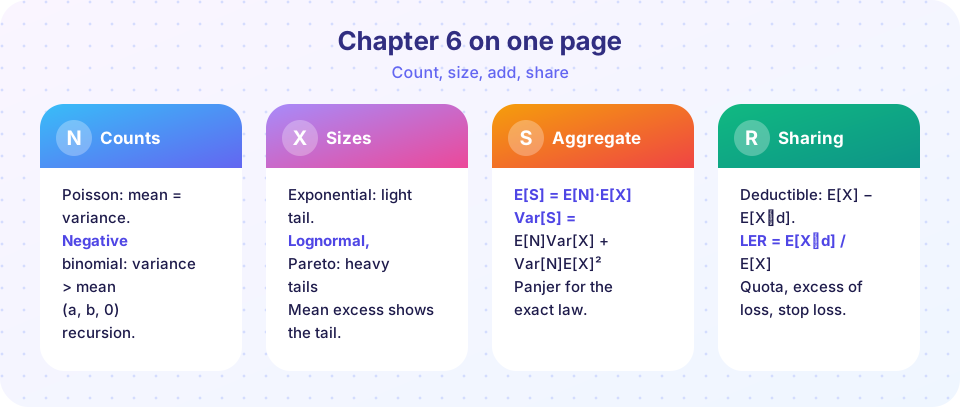
The chapter in one table
| Stage | Key formulas | Watch out for |
|---|---|---|
| Counts | Poisson: E = Var = λ; NB: E = rβ, Var = rβ(1+β) |
Overdispersion: variance above the mean |
| Sizes | Exponential θ; lognormal e^(μ+σ²/2); Pareto θ/(α−1) |
Infinite moments for small α |
| Aggregate | E[S] = E[N]E[X]; Var[S] = E[N]Var[X] + Var[N]E[X]² |
Skew: normal approximation too optimistic |
| Exact law | Panjer: g_s = (λ/s) Σ j f_j g_(s−j) (Poisson) |
Needs discrete claim sizes |
| Deductible | E[(X−d)⁺] = E[X] − E[X∧d]; LER = E[X∧d]/E[X] |
Inflation leverage |
| Reinsurance | Quota q·X; XL (X−M)⁺; stop loss (S−a)⁺ |
Cost of cover versus benefit |
A combined worked example
An insurer writes 500 policies, each with Poisson claim rate 0.2 per year, so λ = 100. Claim sizes are exponential with mean 2,000. The insurer applies a per-claim deductible of 500.
- Counts: the number of claims that exceed the deductible is Poisson with mean
100 × e^(−500/2000) = 100 × e^(−0.25) ≈ 77.9. (Thinning a Poisson count keeps it Poisson.) - Sizes: by the memoryless property, a payment given that the claim exceeds 500 is again exponential with mean 2,000.
- Aggregate payments:
E[S] = 77.9 × 2000 ≈ 155,760, which equals100 × E[(X − 500)⁺] = 100 × 2000 e^(−0.25); the two routes agree.Var[S] = λ' · E[Y²] = 77.9 × 2 × 2000² ≈ 623,000,000, with standard deviation about 24,960. - Sharing: a stop loss at
E[S] + 2σ ≈ 205,700would pay out only in the worst few percent of years.
The code below recomputes each line.
Try it
Press Run (or Ctrl + Enter) to see the result here.
Program input · what you'd type while the program runs
Type the answers before you press Run, one per line. Each time the program reads a line (with input()), it gets the next line from this box.
Press Run (or Ctrl + Enter) to see the result here.
Program input · what you'd type while the program runs
Type the answers before you press Run, one per line. Each time the program reads a line (with input()), it gets the next line from this box.
Common misconceptions
"Frequency and severity can be fitted to totals only." Modelling them separately keeps information about how many claims occurred and how large each was, which is exactly what deductibles and reinsurance act on.
"Thinning a Poisson count by a deductible makes it non-Poisson." If each claim independently exceeds the deductible with probability p, the count of exceeding claims is Poisson with mean pλ.
Check your understanding
Quick check · 10 questions
of 10 answered You scored / 10 · perfect!
-
1. A Poisson claim count has mean 12. Its variance is
For the Poisson, mean and variance are equal. -
2. A negative binomial with r = 4 and β = 0.5 has mean
Mean = rβ = 4 × 0.5 = 2. -
3. The Pareto distribution with α = 0.8 has
The Pareto mean exists only if α > 1. -
4. For compound Poisson with λ = 10 and E[X²] = 500, Var[S] is
Var[S] = λ·E[X²] = 10 × 500 = 5,000. -
5. Which is the correct expected payment per loss with deductible d?
Payment is X − (X ∧ d), whose expectation is E[X] − E[X ∧ d]. -
6. A quota share of 30% means the reinsurer pays
Quota share is proportional: the reinsurer takes a fixed fraction of every claim. -
7. As the number of independent policies n grows, the coefficient of variation of S behaves like
Relative variability shrinks with the square root of the portfolio size. -
8. A mean excess function that increases linearly indicates
The Pareto mean excess is (θ + d)/(α − 1), linear in d. -
9. A deductible of 500 is applied to losses that are exponential with mean 2,000. The expected payment per loss is
E[(X − d)⁺] = θ·e^(−d/θ) = 2000·e^(−0.25). -
10. Which reinsurance form directly caps the insurer's annual total?
Stop loss pays the part of the aggregate above the attachment point.
Summary
- Counts (Poisson, negative binomial) and sizes (exponential, lognormal, Pareto) combine into
S, whose mean and variance follow from conditioning. - Panjer gives the exact law; simulation and the normal approximation give quick checks, with the normal failing in the tail.
- Deductibles, limits and reinsurance are functions of the loss; their values are limited expected values or aggregate expectations.
- Pooling shrinks relative risk but never the systematic risk.
Track your progress
Create a free account to tick off lessons and pick up where you left off on any device.
of Actuarial Mathematics lessons completed