


















Lesson 31 of 43 · Credibility and Ruin Theory
Credibility Theory
Learn how actuaries blend a risk's own claims with the group average: limited fluctuation credibility, Bühlmann credibility, the credibility factor Z and worked examples.
An insurer has a group of similar risks and a rate for the whole group. One member has now had a year with half the expected claims. Should its premium fall by half? Almost never. The sensible answer lies somewhere between the member's own experience and the group's, and credibility theory tells you where.
The idea is old (it was developed for workers' compensation insurance in the early twentieth century) and still central to experience rating, group insurance and the pricing of small portfolios. In this lesson you meet its two classic forms: limited fluctuation credibility, which asks how much data is enough to trust a risk fully, and Bühlmann credibility, which derives the weight from a statistical model.
What you will learn
- Compute the full-credibility standard and partial credibility factor.
- Define the expected process variance and the variance of hypothetical means.
- Compute the Bühlmann credibility factor
Z = n/(n + K)and the credibility premium. - Explain what makes
Zlarge or small.
Key terms
Full credibility: the data are reliable enough that Z = 1.
Expected process variance v: the average variance of a risk's claims around its own mean.
Variance of hypothetical means a: how much the risks' true means differ from each other.
Bühlmann K: the ratio v/a; the number of observations at which Z = 1/2.
Credibility premium: Z · X̄ + (1 − Z) · μ.
Limited fluctuation credibility
The classical approach does not model the differences between risks. It asks: how many claims do I need before the observed average is within a fraction k of the truth with probability p?
For a Poisson number of claims with mean λ, the count is approximately normal with standard deviation √λ. Requiring P(|N − λ| ≤ kλ) ≥ p gives
λ_F = (z / k)² where z is the standard normal quantile (1 + p)/2
With p = 90% and k = 5%, z = 1.645 and λ_F = (1.645/0.05)² ≈ 1,082 claims. If severities also vary, the standard is multiplied by 1 + CV², where CV is the coefficient of variation of claim size. When fewer claims are available, partial credibility uses the square-root rule
Z = min(1, √(n / λ_F))
For example, with 300 expected claims, Z = √(300/1082) ≈ 0.53.
The method is simple and widely used, but it has no explicit model of how risks differ and the square-root rule is a convention. Bühlmann's model fixes this.
Bühlmann credibility
The model
Each risk has a hidden risk parameter Θ drawn from the group's distribution. Given Θ, the annual claim costs X₁, X₂, … are independent with mean m(Θ) and variance s²(Θ). Define
μ = E[m(Θ)], the collective mean;v = E[s²(Θ)], the expected process variance (EPV): noise inside risks;a = Var[m(Θ)], the variance of hypothetical means (VHM): differences between risks.
Then the best linear estimate of the next year's cost, given n years with average X̄, is
estimate = Z · X̄ + (1 − Z) · μ Z = n / (n + K) K = v / a
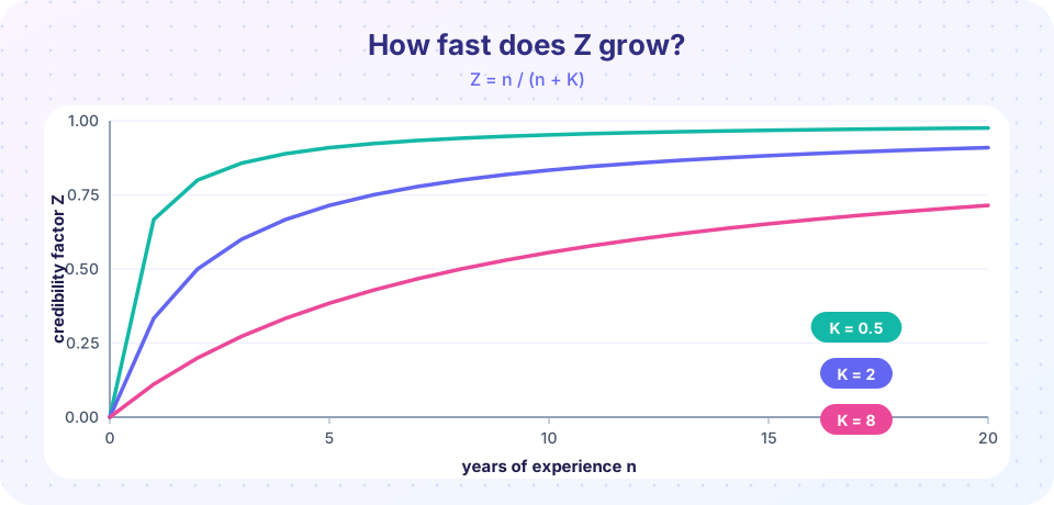
Read it this way: K is a ratio of noise to signal. If risks differ a lot (a large), K is small and few years earn a large Z. If years are noisy (v large), K is large and credibility comes slowly.
Worked example
Two classes of risk: class A (70% of the group) with mean annual cost 100 and variance 2,500; class B (30%) with mean 300 and variance 10,000.
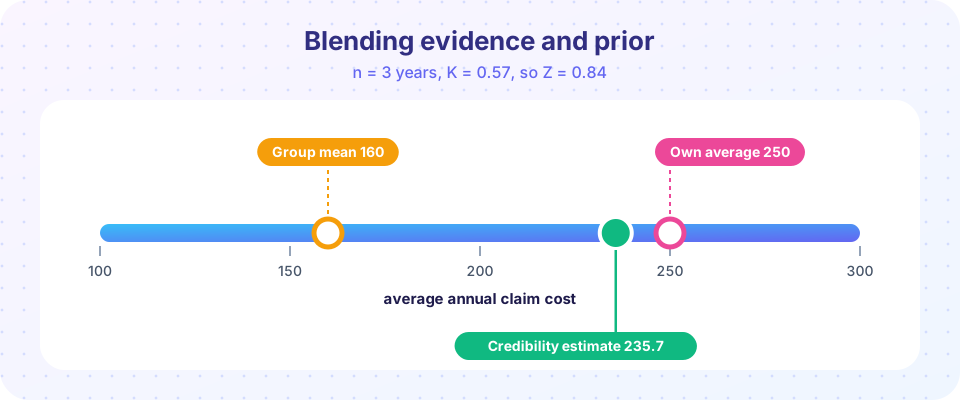
μ = 0.7·100 + 0.3·300 = 160v = 0.7·2500 + 0.3·10000 = 4,750a = 0.7·(100 − 160)² + 0.3·(300 − 160)² = 2,520 + 5,880 = 8,400K = 4750/8400 ≈ 0.566
A risk observed for n = 3 years with average cost 250 has Z = 3/(3 + 0.566) ≈ 0.841 and premium 0.841·250 + 0.159·160 ≈ 235.7. The group mean pulls the estimate down by about 14 from the raw average.
Why it works
Among all estimators of the form α₀ + α₁X₁ + … + αₙXₙ, the Bühlmann estimator has the smallest mean squared error. It is exact (it equals the Bayesian posterior mean) for several standard model pairs, such as Poisson–gamma and normal–normal; for other models it is the best linear approximation.
Try it
Press Run (or Ctrl + Enter) to see the result here.
Program input · what you'd type while the program runs
Type the answers before you press Run, one per line. Each time the program reads a line (with input()), it gets the next line from this box.
Press Run (or Ctrl + Enter) to see the result here.
Program input · what you'd type while the program runs
Type the answers before you press Run, one per line. Each time the program reads a line (with input()), it gets the next line from this box.
Common misconceptions
"Credibility means the data are right or wrong." Z measures how much weight the data deserve relative to the group, not whether they are correct.
"Bühlmann credibility needs a normal distribution." It uses only means and variances; normality is not required.
"The complement of credibility must be the group's overall average." It is the best estimate of what the risk would be without its own data, which may be a related class rate or the previous year's premium.
Check your understanding
Quick check · 5 questions
of 5 answered You scored / 5 · perfect!
-
1. A full credibility standard for p = 90% and k = 5% is about
(1.645/0.05)² ≈ 1,082. -
2. With 541 expected claims and standard 1,082, the square-root partial credibility is about
Z = √(541/1082) = √0.5 ≈ 0.707. -
3. In Bühlmann's model K equals
K is the expected process variance divided by the variance of hypothetical means. -
4. If risks differ more from each other (a gets larger) and v stays the same, Z
K = v/a gets smaller, so Z = n/(n+K) is larger. -
5. With n = 4 and K = 4, Bühlmann Z is
Z = 4/(4 + 4) = 0.5.
Summary
- Limited fluctuation credibility: full standard
(z/k)², partialZ = √(n/λ_F). - Bühlmann credibility:
Z = n/(n + K)withK = v/a; premiumZ·X̄ + (1 − Z)·μ. - Larger differences between risks or less noisy data raise
Z. - Credibility estimates beat both the raw average and the collective mean in mean squared error.
Next: Ruin probability
Track your progress
Create a free account to tick off lessons and pick up where you left off on any device.
of Actuarial Mathematics lessons completed