


















Lesson 42 of 49 · Computational Linguistics
n-gram language models
Learn how n-gram language models predict the next word from counts, why smoothing is needed, how perplexity measures quality, and where these models fall short.
When you type I'll see you at on your phone, it offers the, home or work. Behind that suggestion is a language model: a system that assigns a probability to the next word, given what came before. The oldest and simplest kind is the n-gram model, which looks only at the last few words and estimates probabilities by counting. It is the best way to understand what a language model is, and its weaknesses point directly to modern neural models.
What you will learn
- What a language model computes and how the chain rule decomposes it
- How bigram and trigram probabilities are estimated by counting
- Why smoothing is necessary, with a simple method (add-one) and its alternatives
- What perplexity measures, and where n-grams fail
Key terms
Language model: a probability distribution over sequences of words.
n-gram: a sequence of n words; a bigram model predicts a word from the one before.
Markov assumption: only the last few words matter for predicting the next.
Smoothing: giving some probability to events not seen in training.
Perplexity: a measure of how surprised a model is by test text; lower is better.
From sentences to probabilities
A language model gives a probability to a whole sentence. By the chain rule of probability, this decomposes into a product of predictions:
P(the cat sat) = P(the) × P(cat | the) × P(sat | the cat)
Conditioning on the whole history is hopeless: almost every long history is unique, so we have no counts. The Markov assumption truncates it. A bigram model uses only the previous word:
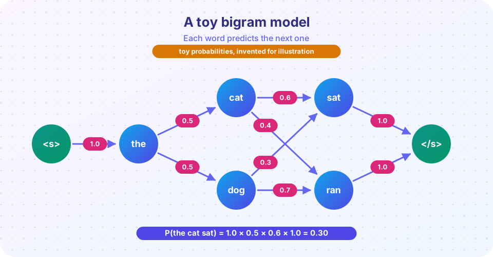
P(the cat sat) ≈ P(the | <s>) × P(cat | the) × P(sat | cat) × P(</s> | sat)
where <s> and </s> mark the sentence start and end. A trigram model uses the previous two words, and so on. Claude Shannon already used such models in 1948 to generate "approximations to English": random text from letter and word frequencies looks more and more like English as the context grows.
Estimating by counting
The maximum-likelihood estimate is just a ratio of counts:
P(cat | the) = count(the cat) / count(the)
If the occurs 100 times in the corpus and the cat 12 times, then P(cat | the) = 0.12. Estimating is trivially fast, which is why n-gram models powered speech recognition and translation for decades. The toy graph above is a bigram model: each arrow's probabilities out of a word sum to one.
The zero problem and smoothing
Zipf's law tells us that most word sequences never appear in training. If a test sentence contains one unseen bigram, the product becomes zero, as if the sentence were impossible. Smoothing moves probability from seen to unseen events.
- Add-one (Laplace) smoothing adds one to every count:
P(w | v) = (count(v w) + 1) / (count(v) + V), where V is the vocabulary size. Simple but it gives too much mass to unseen events in large vocabularies. Add-k with small k is a common variant. - Backoff and interpolation combine higher- and lower-order estimates: if you have never seen the purple, use the unigram probability of purple. Katz backoff and Jelinek-Mercer interpolation follow this idea.
- Kneser-Ney smoothing (Kneser and Ney, 1995) refines the lower-order estimate: it asks not "how often does this word occur?" but "in how many different contexts does it occur?" Francisco is frequent but almost always follows San, so as a fallback it should be rare. Kneser-Ney was the standard for years.
Perplexity
To compare models, evaluate them on held-out test text that was not used in training. The standard measure is perplexity, the inverse probability of the test set normalised by its length:
PP = exp( −(1/N) × Σ log P(w_i | history) )
It can be read as the average number of choices the model is torn between at each step. A model that assigns probability 1/10 to every next word has perplexity 10. Lower perplexity means better prediction. Perplexity numbers are comparable only for the same test set and vocabulary.
What n-grams cannot do
- Long-range dependency. In The keys that the old man left on the table are missing, the verb are agrees with keys, many words back. A trigram model sees only on the table and may prefer is. Syntax is hierarchical, not just local.
- Data hunger. The number of possible n-grams explodes with n, so counts become sparse.
- No meaning. Counting does not capture that cat and kitten are similar; each is just a symbol.
In 1957 Chomsky argued that a statistical model could not tell Colorless green ideas sleep furiously from its reverse, since both are absent from any corpus. Fernando Pereira (2000) answered that a smoothed model trained on text assigns a far higher probability to the first than to the reverse, because it captures category-level regularities. Both authors had a point: statistics can learn some structure, but local counts alone do not capture all of syntax.
Modern language models use neural networks, which represent words as vectors and can use much longer context. But the task is the same: predict the next word, and measure by perplexity or a related score.
Common misconceptions
"A language model understands text." An n-gram model is a table of counts. Larger neural models are more capable, but "predicting the next word well" is a statement about performance, not necessarily about understanding.
"Smoothing is a hack." Estimating from finite data always needs a principled way to handle unseen events; smoothing is that.
"Lower perplexity always means a better application." It correlates with quality, but it is not identical to translation or recognition accuracy.
Try it
The first demo builds bigram counts from a tiny corpus, shows that an unseen sentence gets probability zero, and fixes it with add-one smoothing. The corpus is too small for real use; the point is the mechanics.
Press Run (or Ctrl + Enter) to see the result here.
Program input · what you'd type while the program runs
Type the answers before you press Run, one per line. Each time the program reads a line (with input()), it gets the next line from this box.
The second demo trains unigram, bigram and trigram models on a synthetic corpus and measures perplexity on held-out sentences. The corpus comes from a small random grammar, so real text will behave differently. Compare the bars.
Press Run (or Ctrl + Enter) to see the result here.
Program input · what you'd type while the program runs
Type the answers before you press Run, one per line. Each time the program reads a line (with input()), it gets the next line from this box.
Check your understanding
Quick check · 6 questions
of 6 answered You scored / 6 · perfect!
-
1. What does a bigram model use to predict the next word?
A bigram conditions on one preceding word. -
2. If the occurs 100 times and the cat 12 times, what is the maximum-likelihood estimate of P(cat | the)?
12 divided by 100. -
3. Why is smoothing needed?
Because of Zipf's law, many valid sequences are missing from training data. -
4. What does perplexity measure?
Lower perplexity means better prediction. -
5. Why do n-gram models struggle with The keys that the old man left on the table are missing?
The verb agrees with keys, which lies outside the local window. -
6. What does Kneser-Ney smoothing add to simple backoff?
A word like Francisco that appears in few contexts should be a poor fallback.
Summary
- A language model assigns probabilities to sequences; n-grams estimate them by counting.
- Zipf's law makes zeros common, so smoothing is essential.
- Perplexity on held-out text compares models.
- Local counts miss long-range syntax and meaning, which neural models address.
Next: Tagging and parsing
Track your progress
Create a free account to tick off lessons and pick up where you left off on any device.
of Linguistics lessons completed