


















Lesson 25 of 46 · Viscous Flow and Boundary Layers
The laminar boundary layer and the Blasius solution
Learn Prandtl's boundary-layer idea, solve the Blasius equation for a flat plate, and compute layer thickness, skin friction and drag with worked numbers.
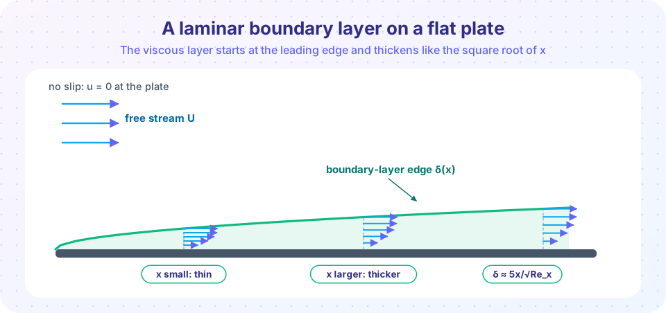
In 1904 Ludwig Prandtl gave a talk in Heidelberg that changed fluid mechanics. His claim: at large Reynolds number, viscous effects are confined to a thin layer next to the body, and outside that layer the flow is ideal. Inside the layer the equations simplify enough to be solved. Three years later his student Paul Richard Heinrich Blasius solved the simplest case, a flat plate aligned with the stream, and the result is still the standard reference for laminar skin friction.
What you will learn
- How scale analysis predicts that the layer thickness is
δ ~ x / √Re_x. - The Blasius similarity solution and its key numbers (0.332, 4.91, 1.72, 0.664).
- How to compute skin friction and the drag on a plate, and how turbulent layers differ.
- How to solve the Blasius equation numerically with a shooting method.
Key terms
- Boundary-layer thickness (δ): the distance from the wall where
ureaches 99% of the free-stream speedU. - Displacement thickness (δ*): how far the outer flow is pushed away from the wall by the slow fluid in the layer.
- Momentum thickness (θ): a measure of the momentum lost in the layer; proportional to the drag.
- Skin friction coefficient (Cf):
Cf = τw / (½ ρ U²). - Local Reynolds number:
Re_x = U x / ν, withxmeasured from the leading edge.
Why the layer is thin: scaling
Let L be the plate length and δ the layer thickness, with δ ≪ L. Fluid in the layer spends a time L/U passing along the plate. During this time, viscous diffusion spreads momentum a distance of order √(ν t) = √(ν L / U). Setting this equal to δ gives
δ / L ~ √(ν / (U L)) = 1 / √Re_L
For air over a 1 m plate at 10 m/s, Re = 6.7 × 10⁵ and δ/L ~ 0.0012, so the layer is about a millimeter thick. The thinness is the whole point. Across a layer this thin, pressure hardly changes (∂p/∂y ≈ 0), so the outer-flow pressure is imposed on the layer. Prandtl's boundary-layer equations are:
- Continuity:
∂u/∂x + ∂v/∂y = 0 - x-momentum:
u ∂u/∂x + v ∂u/∂y = -(1/ρ) dp/dx + ν ∂²u/∂y²
For a flat plate in a uniform stream, dp/dx = 0.
The Blasius solution
Blasius noticed that velocity profiles at different x look the same if y is rescaled by the local thickness. Define the similarity variable and a stream function:
η = y √(U / (ν x)), ψ = √(ν U x) f(η), so u = U f'(η)
The momentum equation then collapses to one ordinary differential equation:
f''' + ½ f f'' = 0, with f(0) = 0, f'(0) = 0, f'(∞) = 1
There is no closed-form solution, but it is easy to integrate numerically. The important results are:
| Quantity | Value |
|---|---|
Wall gradient f''(0) |
0.3321 |
| Thickness (99%) | δ = 4.91 x / √Re_x (often rounded to 5) |
| Displacement thickness | δ* = 1.721 x / √Re_x |
| Momentum thickness | θ = 0.664 x / √Re_x |
| Local friction | Cf = 0.664 / √Re_x |
| Drag on one side of length L | C_D = 1.328 / √Re_L |
Skin friction falls like x^(-1/2) because the layer thickens while the free-stream speed stays the same, so the wall gradient weakens. The total drag grows only like √L. Doubling the length of the plate does not double the drag.
Worked example
Air (ν = 1.5 × 10⁻⁵ m²/s, ρ = 1.2 kg/m³) flows at 3 m/s along a plate 0.5 m long. Then:
Re_L = 3 × 0.5 / (1.5 × 10⁻⁵) = 1.0 × 10⁵, laminar.δ(L) = 4.91 × 0.5 / √(10⁵) = 7.8 mm.C_D = 1.328 / 316.2 = 4.2 × 10⁻³.- Drag per meter of width, one side:
D = C_D × ½ ρ U² × L = 0.0042 × 5.4 × 0.5 ≈ 0.011 N/m.
Turbulent boundary layers
If the layer becomes turbulent, it grows faster and the wall friction is larger. Common empirical power-law fits, valid for 5 × 10⁵ ≲ Re_x ≲ 10⁷, are δ ≈ 0.37 x Re_x^(-1/5) and Cf ≈ 0.0576 Re_x^(-1/5), with C_D ≈ 0.074 Re_L^(-1/5) if the layer is turbulent from the leading edge. The turbulent layer grows like x^(4/5), much faster than the laminar x^(1/2). Chapter 6 explains why turbulence has this effect.
When does a laminar layer become turbulent? Linear stability theory finds that small disturbances begin to grow (Tollmien-Schlichting waves) at Re_x ≈ 9 × 10⁴ (Re_δ* ≈ 520), but complete transition on real plates usually happens between 3 × 10⁵ and 3 × 10⁶, depending on free-stream turbulence and roughness. Many textbooks use 5 × 10⁵ as a working value.
Limits of the flat-plate result
The Blasius solution needs three things: no pressure gradient, a smooth plate, and a thin layer. Near the leading edge, where Re_x is small, the thin-layer assumption breaks down. If the outer flow decelerates (a rising pressure, as on the back of a body), the layer thickens quickly and can separate, which is the topic of the next lesson.
Common misconceptions
- "The boundary layer edge is a solid line." The 99% definition is a convention. Velocity approaches
Ugradually, so the edge is a matter of definition. - "A thicker layer means more drag." Along a laminar plate the layer gets thicker while the local friction falls. Friction depends on the wall gradient, not on thickness itself.
- "Boundary layers need turbulence." A laminar layer is perfectly valid and is the starting point of every layer.
Try it
Press Run (or Ctrl + Enter) to see the result here.
Program input · what you'd type while the program runs
Type the answers before you press Run, one per line. Each time the program reads a line (with input()), it gets the next line from this box.
Press Run (or Ctrl + Enter) to see the result here.
Program input · what you'd type while the program runs
Type the answers before you press Run, one per line. Each time the program reads a line (with input()), it gets the next line from this box.
The first two examples apply the formulas of this lesson. The slider is a calculator, not a flow simulation.
Check your understanding
Quick check · 5 questions
of 5 answered You scored / 5 · perfect!
-
1. How does the laminar boundary-layer thickness on a flat plate grow with distance x?
δ = 4.91 x / √Re_x ∝ √x for a laminar layer. The 4/5 power describes a turbulent layer. -
2. Doubling the speed U of the stream over a plate changes the laminar thickness at a fixed x by what factor?
δ ∝ 1/√Re_x ∝ 1/√U, so doubling U divides δ by √2. -
3. What is the local skin friction coefficient on a laminar plate?
Cf = 0.664/√Re_x for the Blasius layer. The second expression is a turbulent fit and the third is for pipes. -
4. Which assumption does the Blasius solution rely on?
dp/dx = 0 for uniform flow along a flat plate; this lets the problem reduce to the single Blasius ODE. -
5. Why does the total laminar drag grow only like √L?
Integrating Cf ∝ x^(-1/2) along the plate gives a total proportional to L^(1/2).
Summary
- Scale analysis gives
δ/L ~ 1/√Re_L; the layer is thin at high Reynolds number. - The Blasius similarity solution yields
δ = 4.91 x/√Re_x,Cf = 0.664/√Re_xandC_D = 1.328/√Re_L. - Turbulent layers grow faster and give more skin friction.
- The result holds for zero pressure gradient; pressure gradients change everything.
Track your progress
Create a free account to tick off lessons and pick up where you left off on any device.
of Fluid Dynamics lessons completed