


















Lesson 38 of 46 · Computational Fluid Dynamics
Finite differences, stability and numerical diffusion
Discretize advection and diffusion with finite differences, learn the CFL and diffusion stability limits, see numerical diffusion and measure the order of accuracy.
The Navier-Stokes equations combine two very different transport processes. Advection carries a quantity along with the flow, and diffusion spreads it out. The simple model equation ∂u/∂t + c ∂u/∂x = ν ∂²u/∂x² contains both, and it is the best laboratory for learning how numerical methods behave. The lessons here (stability limits, numerical diffusion, order of accuracy) carry over to the full equations.
What you will learn
- How finite differences come from Taylor series and what truncation error means.
- The stability limits
r = ν Δt/Δx² ≤ 1/2andCFL = c Δt/Δx ≤ 1. - Why upwind schemes smear (numerical diffusion) and why second-order schemes oscillate.
- How to measure the order of accuracy by refining the grid.
Key terms
- Truncation error: the error from cutting off the Taylor series, such as
O(Δx)orO(Δx²). - Order of accuracy: if the error is proportional to
Δx^p, the scheme has orderp. - Stability: errors (including rounding) do not grow without bound.
- CFL number:
c Δt / Δx, the fraction of a cell that information crosses in one time step. - Numerical diffusion: smoothing introduced by the scheme itself.
Differences from Taylor series
On a uniform grid x_j = jΔx, expand u(x ± Δx) about x_j:
u_{j+1} = u_j + Δx u' + ½Δx² u'' + ⅙Δx³ u''' + ...
Subtracting the corresponding equation for u_{j-1} gives the central difference
u'(x_j) ≈ (u_{j+1} - u_{j-1}) / (2Δx), with error O(Δx²).
The backward difference (u_j - u_{j-1})/Δx has error O(Δx). Adding the two expansions gives the second derivative:
u''(x_j) ≈ (u_{j+1} - 2u_j + u_{j-1}) / Δx², with error O(Δx²).
Diffusion: the explicit scheme and its limit
For u_t = ν u_xx the explicit (forward Euler in time, central in space) scheme is
u_j^{n+1} = u_j^n + r (u_{j+1}^n - 2u_j^n + u_{j-1}^n), with r = ν Δt / Δx²
To test stability, von Neumann analysis inserts a Fourier mode u_j^n = G^n e^{i k j Δx}. The amplification factor is G = 1 - 4r sin²(kΔx/2). For the mode with the shortest wavelength, sin² = 1 and G = 1 - 4r. We need |G| ≤ 1, so
r ≤ 1/2
If you halve Δx to improve accuracy, you must cut Δt by four. Fully implicit schemes (backward Euler) are stable for any r but require solving a tridiagonal system each step, a good trade for stiff problems.
Advection: upwind and Lax-Wendroff
For u_t + c u_x = 0 with c > 0, three natural schemes are:
| Scheme | Formula | Accuracy | Stability |
|---|---|---|---|
| Central in space, forward in time | u_j - (CFL/2)(u_{j+1} - u_{j-1}) |
O(Δt, Δx²) |
unstable for every CFL |
| First-order upwind | u_j - CFL (u_j - u_{j-1}) |
O(Δt, Δx) |
stable for 0 ≤ CFL ≤ 1 |
| Lax-Wendroff | central plus (CFL²/2)(u_{j+1} - 2u_j + u_{j-1}) |
O(Δt², Δx²) |
stable for CFL ≤ 1 |
Upwinding means using the points from which the information comes: for c > 0, the flow comes from the left, so we use u_{j-1}. It follows the physics of the equation. The CFL condition (Courant, Friedrichs and Lewy, 1928) has a clear meaning: in one time step the numerical domain of dependence must include the physical one, so information cannot travel more than one cell per step.
Numerical diffusion
What equation does the upwind scheme actually solve? Expanding its terms in Taylor series gives the modified equation
u_t + c u_x = (c Δx / 2)(1 - CFL) u_xx + ...
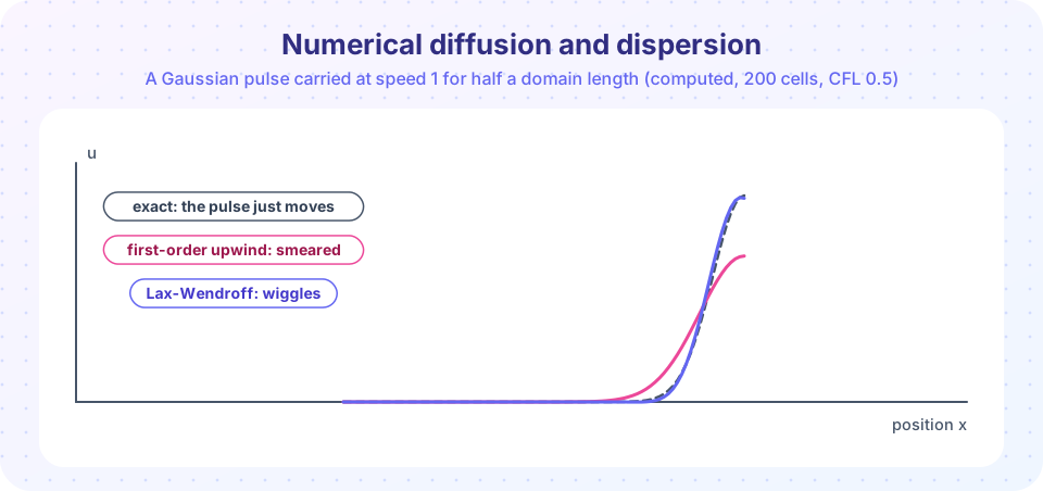
The right side is a diffusion term with a coefficient ν_num = c Δx (1 - CFL)/2 that comes from the scheme alone. That is why the pulse in the picture is lower and broader. Numerical diffusion can easily exceed the physical diffusion, and it hides real physics such as thin shear layers. At CFL = 1 the upwind scheme is exact for pure advection, the only case without it.
Lax-Wendroff removes the diffusion at second order but leaves a dispersive error: short wavelengths travel at the wrong speed, producing oscillations (wiggles) near sharp features. Godunov's theorem says that no linear scheme of order higher than one can be monotone. The way out is nonlinear limiters (flux limiters, TVD, WENO), used in all modern shock and high-Reynolds codes.
Cell Péclet number
With both processes present, central differencing of advection stays well behaved only if the cell Péclet number Pe = c Δx / ν is at most 2. For Pe > 2 it produces non-physical oscillations and upwinding (or finer cells) is needed. This is the main reason that high-Reynolds-number CFD uses upwind-biased or limited schemes.
Common misconceptions
- "A stable scheme is an accurate scheme." Upwind is stable but only first-order accurate and smears.
- "If the code runs without blowing up, the answer is right." A convergent solution of the wrong problem is common. Check against an exact solution.
- "Smaller Δt always helps." For explicit schemes smaller Δt is stable but adds cost. Accuracy is limited by
Δxif time errors are already small.
Try it
Press Run (or Ctrl + Enter) to see the result here.
Program input · what you'd type while the program runs
Type the answers before you press Run, one per line. Each time the program reads a line (with input()), it gets the next line from this box.
Press Run (or Ctrl + Enter) to see the result here.
Program input · what you'd type while the program runs
Type the answers before you press Run, one per line. Each time the program reads a line (with input()), it gets the next line from this box.
Press Run (or Ctrl + Enter) to see the result here.
Program input · what you'd type while the program runs
Type the answers before you press Run, one per line. Each time the program reads a line (with input()), it gets the next line from this box.
On coarse grids the measured order of upwind is below one because the pulse is barely resolved; it approaches one as the mesh is refined, while Lax-Wendroff reaches two. Order only means something in the range where the grid resolves the solution.
Check your understanding
Quick check · 5 questions
of 5 answered You scored / 5 · perfect!
-
1. What is the stability limit of the explicit scheme for u_t = ν u_xx?
Von Neumann analysis gives G = 1 - 4r sin²(kΔx/2), and |G| ≤ 1 requires r ≤ 1/2. -
2. If you halve Δx in an explicit diffusion calculation, how must Δt change to keep r fixed?
r = νΔt/Δx², so Δt must scale with Δx². -
3. Why does first-order upwind smear sharp pulses?
The modified equation contains (cΔx/2)(1 - CFL) u_xx, a numerical diffusion. -
4. What does the CFL condition require?
The numerical domain of dependence must contain the physical one: c Δt/Δx ≤ 1 for these schemes. -
5. A scheme's error drops by a factor of 4 when Δx is halved. What is its order?
Error ∝ Δx^p gives 2^p = 4, so p = 2.
Summary
- Finite differences come from Taylor series; central differences are second-order accurate.
- Explicit diffusion needs
r ≤ 1/2; advection schemes needCFL ≤ 1. - Upwind is stable and smears (
ν_num = cΔx(1-CFL)/2); Lax-Wendroff is sharper but oscillates. - Measure order of accuracy by halving the mesh and watching the error.
Track your progress
Create a free account to tick off lessons and pick up where you left off on any device.
of Fluid Dynamics lessons completed