


















Lesson 19 of 46 · Ideal and Potential Flow
Stream Function and Velocity Potential
Learn the stream function and velocity potential for 2D flow, how to get velocities from them, why they are orthogonal and how psi gives flow rate.
A 2D flow has two velocity components, u and v, plus the pressure to worry about. Two clever scalar functions replace these. The stream function ψ automatically satisfies mass conservation, so it removes one unknown at once. The velocity potential φ automatically satisfies zero vorticity. When a flow is both incompressible and irrotational, each one obeys Laplace's equation, and the curves ψ = const and φ = const form a perfect crisscross grid. This is the key tool of classical aerodynamics.
What you will learn
- How to define
ψandφand recover the velocity from each. - The conditions under which each exists.
- Why the two families of curves are orthogonal.
- How the difference of
ψbetween two streamlines gives a volume flow rate.
Key terms
Stream function ψ(x, y): defined by u = ∂ψ/∂y, v = −∂ψ/∂x; exists for 2D incompressible flow.
Velocity potential φ(x, y): defined by u = ∂φ/∂x, v = ∂φ/∂y; exists for irrotational flow.
Equipotential line: a curve of constant φ.
Laplace's equation: ∇²ψ = 0 and ∇²φ = 0 for flow that is both incompressible and irrotational.
The stream function
For 2D incompressible flow, ∂u/∂x + ∂v/∂y = 0. This is exactly the condition that u dy − v dx is the differential of some function ψ: dψ = u dy − v dx. Hence
u = ∂ψ/∂y, v = −∂ψ/∂x.
Substituting into continuity: ∂²ψ/∂x∂y − ∂²ψ/∂y∂x = 0 for any smooth ψ. Mass conservation is satisfied automatically.
Three facts make ψ useful:
- Lines of constant
ψare streamlines. Along a curve withψ = const,dψ = 0givesdy/dx = v/u: exactly the streamline equation. - Differences give flow rate. The volume flow rate per unit depth between two streamlines
ψ₁andψ₂isQ' = ψ₂ − ψ₁(m²/s). Closely spaced streamlines mean fast flow. - Vorticity connects to
∇²ψ:ω_z = ∂v/∂x − ∂u/∂y = −∇²ψ. If the flow is irrotational,ψsatisfies Laplace's equation.
In polar coordinates: u_r = (1/r) ∂ψ/∂θ, u_θ = −∂ψ/∂r.
The velocity potential
If the flow is irrotational, ∂v/∂x − ∂u/∂y = 0, which is the condition that u dx + v dy is the differential of a function φ: u = ∂φ/∂x, v = ∂φ/∂y, or u = ∇φ. Then incompressibility ∇·u = 0 gives ∇²φ = 0. The potential exists in 3D as well; the stream function does not (in 3D one needs vector potentials, or axisymmetry restricts it again). In polar coordinates: u_r = ∂φ/∂r, u_θ = (1/r) ∂φ/∂θ.
Orthogonality
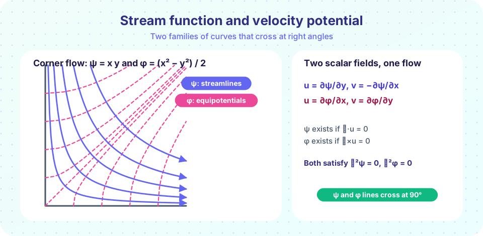
When both functions exist, ∇ψ = (−v, u) and ∇φ = (u, v). Their dot product is −vu + uv = 0. The gradients are perpendicular, so the curves ψ = const and φ = const cross at right angles. Together they form an orthogonal grid called a flow net, a method used by engineers before computers to estimate seepage under dams.
There is an elegant bridge to complex numbers. Writing z = x + iy, any analytic function w(z) = φ + iψ (the complex potential) gives a possible potential flow, because the Cauchy-Riemann equations are exactly the relations above. For example, w = z²/2 = (x² − y²)/2 + i xy gives φ = (x² − y²)/2 and ψ = xy. We study this flow next.
Worked example 1: corner flow ψ = xy
u = ∂ψ/∂y = x, v = −∂ψ/∂x = −y. Check continuity: 1 − 1 = 0 ✓. Vorticity: ∂v/∂x − ∂u/∂y = 0 − 0 = 0 ✓ irrotational. Potential: ∂φ/∂x = x gives φ = x²/2 + g(y), and ∂φ/∂y = −y gives g = −y²/2: φ = (x² − y²)/2. Streamlines xy = c are hyperbolas, and the lines x = 0, y = 0 are streamlines too (ψ = 0), so the axes can be treated as walls: fluid coming down along the y axis spreads out along the x axis. This is the flow of a stagnation point on a wall.
Flow rate between the streamlines ψ = 2 and ψ = 5: Q' = 3 m²/s per metre of depth.
Worked example 2: a rotated corner
Take ψ = x² − y². Then u = −2y, v = −2x. Continuity: 0 + 0 = 0 ✓. Vorticity: −2 − (−2) = 0 ✓. Potential: ∂φ/∂x = −2y so φ = −2xy + g(y), and ∂φ/∂y = −2x forces g' = 0: φ = −2xy. This is the same stagnation-point flow as before, just rotated by 45° and scaled. Note how the roles of ψ and φ swap: the family x² − y² = const is streamlines here and equipotentials there.
Worked example 3: when ψ is not harmonic
The solid-body rotation u = −Ωy, v = Ωx has ∂u/∂x + ∂v/∂y = 0, so it has a stream function: ψ = −Ω(x² + y²)/2. But ∇²ψ = −2Ω = −ω_z, not zero: the flow is rotational and has no velocity potential. Always check which functions exist.
Common misconceptions
"A flow with a stream function is irrotational." The stream function exists for any 2D incompressible flow, rotational or not. Only if ∇²ψ = 0 is the flow irrotational.
"The potential φ is a pressure." It is not. φ is a mathematical device whose gradient is the velocity. Pressure follows afterwards from Bernoulli's equation.
"Streamlines and equipotentials always cross at right angles." Only when both exist, i.e. in a flow that is both incompressible and irrotational.
Try it
First let sympy do the algebra for a few flows: compute u and v from ψ, check continuity and vorticity, and test whether ψ is harmonic.
Press Run (or Ctrl + Enter) to see the result here.
Program input · what you'd type while the program runs
Type the answers before you press Run, one per line. Each time the program reads a line (with input()), it gets the next line from this box.
Second, draw the flow net for ψ = xy, φ = (x² − y²)/2. Each cell of the net is nearly a square, a sign of a good flow net.
Press Run (or Ctrl + Enter) to see the result here.
Program input · what you'd type while the program runs
Type the answers before you press Run, one per line. Each time the program reads a line (with input()), it gets the next line from this box.
Third, the speed and flow rate from ψ in the console. The numbers confirm that crowded streamlines carry fast flow.
Press Run (or Ctrl + Enter) to see the console output here.
No output.
Check your understanding
Quick check · 5 questions
of 5 answered You scored / 5 · perfect!
-
1. The stream function is defined by
u = d psi / d y and v = - d psi / d x; this automatically satisfies the incompressible continuity equation. -
2. For psi = 4xy, the velocity components are
u = dpsi/dy = 4x and v = -dpsi/dx = -4y. -
3. The volume flow rate per unit depth between streamlines psi = 3 and psi = 7 is
The difference psi_2 - psi_1 = 4 m^2/s. -
4. Streamlines and equipotential lines are perpendicular because
grad psi = (-v, u) and grad phi = (u, v), whose dot product is zero. -
5. A flow has a stream function but no velocity potential. It must be
psi exists for any 2D incompressible flow; phi exists only if the flow is also irrotational.
Summary
ψ(u = ψ_y,v = −ψ_x) exists for 2D incompressible flow; its level curves are streamlines and its differences are flow rates.φ(u = ∇φ) exists for irrotational flow; both satisfy Laplace's equation when both exist.- Streamlines and equipotentials form an orthogonal net;
w = φ + iψis an analytic function ofz. - Always check continuity and vorticity before assuming either function exists.
Track your progress
Create a free account to tick off lessons and pick up where you left off on any device.
of Fluid Dynamics lessons completed