


















Lesson 7 of 46 · Continuum and Kinematics
Eulerian and Lagrangian Views, and the Material Derivative
Two ways to describe a flow, at fixed points or following particles, and the material derivative D/Dt that links them, with worked numbers for a river and a nozzle.
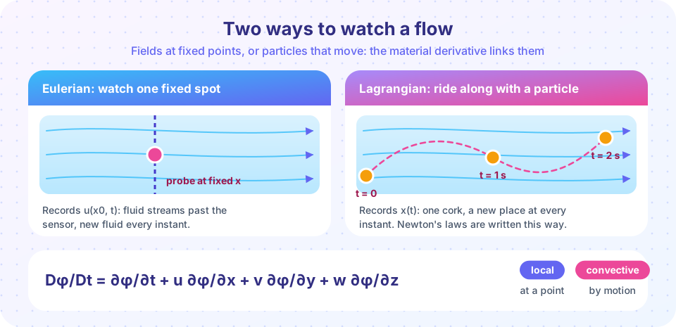
There are two natural ways to watch a river. You can stand on a bridge with a speed gun and record how fast the water moves under you, minute after minute. Or you can drop a cork in and follow it downstream. These two viewpoints have names, after two great eighteenth-century mathematicians: Leonhard Euler, who favored fields at fixed points, and Joseph-Louis Lagrange, who favored following particles. Newton's second law is naturally Lagrangian (it talks about the acceleration of a piece of matter), but fields are far more convenient to work with. The material derivative is the bridge.
What you will learn
- The difference between the Eulerian and Lagrangian descriptions.
- How to compute the material derivative of a scalar and the acceleration of a fluid particle.
- Why a steady flow can still have acceleration.
- How to compute a rate of change seen by a moving sensor.
Key terms
Eulerian view: quantities are functions of position and time, φ(x, y, z, t).
Lagrangian view: quantities are followed along each particle's path, φ(t) for a named particle.
Local derivative ∂φ/∂t: the rate of change at a fixed point.
Convective derivative u·∇φ: the change because the particle moves to a place where φ is different.
Material derivative Dφ/Dt = ∂φ/∂t + u·∇φ: the rate of change following a particle.
The two views
In the Eulerian description the unknowns are fields. A probe fixed at position x0 records u(x0, t), whichever fluid is passing. The advantage: we usually care about what happens in a given place (a pipe junction, a wing surface), not about the history of individual particles, and fields have well-developed mathematics.
In the Lagrangian description we label each particle by where it started, x0, and track its position x(x0, t). Newton's law is simple here: mass times the second time derivative of position equals force. But with trillions of particles the bookkeeping is overwhelming, except in a few problems (a single droplet, a bubble, a tracer in a lab).
From fields to particles: the material derivative
Let φ(x, y, z, t) be any field, such as temperature. A particle moves along a path x(t), y(t), z(t) with velocity (u, v, w) = (dx/dt, dy/dt, dz/dt). The temperature it feels is φ(x(t), y(t), z(t), t). By the chain rule:
Dφ/Dt = ∂φ/∂t + u ∂φ/∂x + v ∂φ/∂y + w ∂φ/∂z = ∂φ/∂t + (u · ∇)φ.
The capital D reminds us that we follow the fluid. Two effects can change what a particle feels: the field itself may change in time (∂φ/∂t, local), or the particle may be carried to a place where the field has a different value (u·∇φ, convective).
Apply this to the velocity itself and you get the acceleration of a fluid particle:
a = Du/Dt = ∂u/∂t + (u·∇)u.
In components, a_x = ∂u/∂t + u ∂u/∂x + v ∂u/∂y + w ∂u/∂z, and similarly for y and z. The second term is nonlinear, because velocity multiplies its own derivative. This single term is the source of almost all of the mathematical difficulty of fluid dynamics, including turbulence.
Worked example 1: a boat on a river
The water temperature along a river increases downstream at a steady 0.002 °C per metre (so ∂T/∂x = 0.002 K/m) and does not change in time at any point (∂T/∂t = 0). A boat drifts with the water at u = 2 m/s. What temperature change rate does a thermometer on the boat read?
DT/Dt = ∂T/∂t + u ∂T/∂x = 0 + 2 × 0.002 = 0.004 K/s.
That is 0.24 K per minute. A fixed thermometer reads no change at all, yet a drifting one reads steady warming. The difference is entirely the convective term.
Worked example 2: acceleration in a steady nozzle
In a converging nozzle the speed along the axis rises linearly: u(x) = u₀ (1 + x/L) with u₀ = 2 m/s and L = 1 m. The flow is steady, so ∂u/∂t = 0. Yet particles speed up:
a = u du/dx = u₀ (1 + x/L) × u₀/L = u₀² (1 + x/L) / L.
At x = 1 m: u = 4 m/s and a = 4 × 2 / 1 = 8 m/s². A fluid particle entering the nozzle at x = 0 is accelerated even though the pattern of the flow never changes. Because a > 0 somewhere, a force must push the fluid: that force is a pressure difference, as chapter 4 will show.
Worked example 3: the case with no convection
If the velocity is uniform in space but changes in time, say u = U sin(ωt) everywhere (an oscillating piston pushing fluid in a wide tube), then (u·∇)u = 0 and a = ∂u/∂t = Uω cos(ωt). Here the local and material derivatives are the same.
Common misconceptions
"Steady flow means zero acceleration." Steady means ∂/∂t = 0. Particles can still accelerate by moving through a spatially varying field: in a nozzle, around a bend, past a cylinder.
"∂φ/∂t and Dφ/Dt are just two notations." They are different quantities. ∂φ/∂t is the change at a point; Dφ/Dt is the change on a particle. They agree only if the flow does not carry the particle to a place with a different value.
"The Eulerian view ignores particles." Fields describe the average of very many particles; the material derivative is exactly how particle physics enters.
Try it
First, verify worked example 2 symbolically with sympy and compare what a fixed probe sees with what a particle sees. The fixed probe at x = 0.5 m always reads 3 m/s; the particle released at x = 0 speeds up exponentially.
Press Run (or Ctrl + Enter) to see the result here.
Program input · what you'd type while the program runs
Type the answers before you press Run, one per line. Each time the program reads a line (with input()), it gets the next line from this box.
Second, an animation of the same nozzle. The blue probe stays put and reports a constant speed; the pink particle moves along the axis and its reading grows. Press the button to release a new particle.
Third, the river thermometer in the console: the material derivative from finite differences.
Press Run (or Ctrl + Enter) to see the console output here.
No output.
Check your understanding
Quick check · 5 questions
of 5 answered You scored / 5 · perfect!
-
1. The material derivative of a field phi is
Dphi/Dt = partial phi / partial t + (u . grad) phi: local change plus convective change. -
2. A steady flow has du/dx = 3 per second and speed u = 4 m/s at a point. The convective acceleration is
a = u du/dx = 4 x 3 = 12 m/s^2, even though the flow is steady. -
3. Which description is best for applying Newton's second law to a small piece of fluid?
Newton's law concerns the acceleration of a piece of matter, which is the material derivative Du/Dt. -
4. A thermometer drifts with the water at 3 m/s. Temperature does not change in time at any point and rises downstream at 0.001 K/m. What does it read?
DT/Dt = 0 + 3 x 0.001 = 0.003 K/s. -
5. For u = U sin(omega t) uniform in space, the acceleration of a fluid particle is
With no spatial variation the convective term vanishes, leaving a = du/dt = U omega cos(omega t).
Summary
- Eulerian: fields at fixed points. Lagrangian: follow particles.
Dφ/Dt = ∂φ/∂t + u·∇φconnects them; the fluid particle's acceleration isDu/Dt = ∂u/∂t + (u·∇)u.- The convective term is nonlinear and lets steady flows have acceleration.
- Newton's second law is Lagrangian; solving flows is usually done with Eulerian fields.
Track your progress
Create a free account to tick off lessons and pick up where you left off on any device.
of Fluid Dynamics lessons completed