


















Lesson 35 of 49 · Radiation and Antennas
Retarded potentials and finite signal speed
Solve the potential wave equations with sources, understand retarded time and the Lienard-Wiechert potentials, and compute retardation for a moving charge.
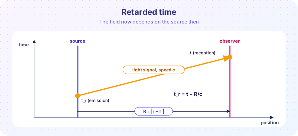
In electrostatics, Coulomb's law gives V = (1/4πε₀) ∫ ρ/𝔯 dτ, with 𝔯 the distance from source to field point. This treats the source as acting instantly across any distance. But Maxwell's theory has a built-in finite speed: if you wiggle a charge on the Sun, Earth will not know for 499 seconds. The correct solution replaces the charge distribution at time t with the distribution at the retarded time.
What you will learn
- Write the retarded solutions for
VandA. - Compute the retarded time for given positions.
- State the Liénard-Wiechert potentials of a point charge.
- Explain why
t_rdepends on the source's motion.
Key terms
Retarded time t_r = t − |r − r'|/c. Retarded potentials: solutions of □V = −ρ/ε₀, □A = −μ₀J that depend only on earlier source values. Source point r', field point r. Separation vector 𝔯 = r − r'. Liénard-Wiechert potentials: the retarded potentials of a moving point charge.
The retarded solutions
Chapter 5 gave □V = −ρ/ε₀ and □A = −μ₀J in Lorenz gauge. When there are no time dependences, the solutions are the usual Coulomb and Biot-Savart integrals. The general solution that respects causality is
V(r, t) = (1/4πε₀) ∫ ρ(r', t_r) / |r − r'| dτ'
A(r, t) = (μ₀/4π)  ∫ J(r', t_r) / |r − r'| dτ'
t_r = t − |r − r'|/c
Every source element contributes with a delay equal to its light-travel time to the field point. You could also write an "advanced" solution using t + |r − r'|/c, which satisfies the same equation but would have effects precede causes, so we discard it.
Why this works: a derivation in four steps
You do not have to take the formula on faith. Here is how it arises.
- Start from the static case. For a time-independent charge density,
∇²V = −ρ/ε₀has the solution that sumsρ dτ' /(4πε₀ 𝔯): each little charge makes a1/𝔯potential. - Look for a spherical wave from a point source. Away from the source the wave equation
∇²V − (1/c²) ∂²V/∂t² = 0has spherically symmetric solutionsV = f(t − r/c)/r, an outgoing wave of any shapef. (Check: forg = rVthe equation reduces to the 1D wave equation∂²g/∂r² = (1/c²) ∂²g/∂t², whose solutions aref(t − r/c)andh(t + r/c).) - Match the static limit near the source. As
r → 0the potential must look like the Coulomb potential of the instantaneous charge,q(t)/(4πε₀ r). Sof(t) = q(t)/(4πε₀), and the outgoing solution isV = q(t − r/c)/(4πε₀ r). - Superpose. The equation is linear, so any charge distribution is a sum of point sources, each evaluated at its own retarded time. That is the integral above. The same argument works for each component of
A.
The other root, h(t + r/c)/r, is the advanced wave: one that converges onto the source. Mathematically it is just as good. Physically we never see waves that converge onto a point in perfect timing, so we pick the retarded root and say that effects follow causes.
Consistency with the Lorenz gauge
The retarded V and A satisfy the Lorenz condition ∇·A + (1/c²) ∂V/∂t = 0 provided charge is conserved (∇·J + ∂ρ/∂t = 0). Conservation of charge is what keeps the potentials consistent, and the fields built from them, E = −∇V − ∂A/∂t and B = ∇×A, then satisfy all four Maxwell equations. Explicit formulas for E and B directly in terms of retarded sources were written down by Oleg Jefimenko in 1966; they show that the fields contain the time derivative of the sources at the retarded time, which is where the acceleration dependence of radiation hides.
Delays in practice
| Path | Distance | Delay |
|---|---|---|
| Across a room | 5 m | 17 ns |
| Geostationary satellite | 3.6 × 10⁷ m | 0.12 s |
| Moon | 3.84 × 10⁸ m | 1.28 s |
| Sun | 1.496 × 10¹¹ m | 499 s |
Moving point charges
For a point charge q on a path w(t) the integral over ρ is not trivial: the charge may move while the signal travels, so the "effective volume" differs from the charge volume. The result is the Liénard-Wiechert potentials
V(r, t) = q / (4πε₀) × 1 / (𝔯 − 𝔯·v/c)
A(r, t) = (v/c²) V(r, t)
with 𝔯, v and everything evaluated at the retarded time t_r. The factor 1 − 𝔯̂·v/c is the Doppler-like squeeze: a charge approaching the observer at nearly c has a much stronger potential. The t_r is found by solving |r − w(t_r)| = c(t − t_r).
Worked example: circular motion
A charge circles at radius a = 1 m with period T = 2π/ω. The field point is on the axis at z = 3 m. The distance from every point on the circle to the field point is √(a² + z²) = √10 = 3.162 m, so the retarded time is simply t − 3.162/c = t − 10.5 ns. Off-axis it requires iteration; the TryIt solves it numerically.
The potentials were found by Alfred-Marie Liénard (1898) and Emil Wiechert (1900), before relativity was formulated. Their result already contained the relativistic factors, a hint that electrodynamics and relativity belong together, which is the subject of Chapter 8.
Worked example: a fast charge passing by
Let a charge q move along a straight line at v = βc and pass its closest point to an observer, at distance b, exactly at t = 0. What is V at the observer at that moment?
- The retarded condition is
c(0 − t_r) = √(v²t_r² + b²). Square it:c²t_r²(1 − β²) = b², so|t_r| = γ b / cwithγ = 1/√(1 − β²). The signal left when the charge wasβγbbefore its closest point. - The separation at that time is
𝔯 = cγb/c = γb. - The velocity component along the line of sight:
𝔯̂·v/c: the unit vector from charge to observer has components(β, 1/γ)in (along-track, perpendicular), so𝔯̂·β = β². - The denominator is
𝔯(1 − 𝔯̂·β) = γb(1 − β²) = b/γ, soV = q γ /(4πε₀ b).
A naive Coulomb formula with the present distance would give q/(4πε₀ b). The retarded result is larger by the Lorentz factor, γ: for β = 0.9 that is γ = 2.29. For a 1 nC charge at b = 1 m the potential is about 20.6 V instead of 9.0 V. The TryIt confirms this numerically.
"The retarded time is a fixed delay." It depends on where the source was: for a moving charge you must solve an implicit equation for t_r.
"Fields propagate instantly in electrostatics, so retarded effects are small corrections." In radiation they are the whole story; the 1/r radiation field exists only because of retardation.
"The advanced solution is wrong mathematically." It is a valid solution; it is excluded by causality (and by the arrow of time defined by sources).
"The field of a moving charge points to where the charge is now." It points to where the charge would be now if it had kept moving uniformly since the retarded time. For uniform motion that happens to be the present position (a surprising result), but if the charge accelerates the field still points to the extrapolated position, not the actual one. That mismatch is the kink of the overview.
Try it
Press Run (or Ctrl + Enter) to see the result here.
Program input · what you'd type while the program runs
Type the answers before you press Run, one per line. Each time the program reads a line (with input()), it gets the next line from this box.
Press Run (or Ctrl + Enter) to see the result here.
Program input · what you'd type while the program runs
Type the answers before you press Run, one per line. Each time the program reads a line (with input()), it gets the next line from this box.
Press Run (or Ctrl + Enter) to see the result here.
Program input · what you'd type while the program runs
Type the answers before you press Run, one per line. Each time the program reads a line (with input()), it gets the next line from this box.
Check your understanding
Quick check · 6 questions
of 6 answered You scored / 6 · perfect!
-
1. The retarded time for a source 600 m from the field point is
t_r = t − 600/(3 × 10⁸) = t − 2 µs. -
2. Why are the advanced solutions discarded?
They solve the equation mathematically, but violate causality. -
3. In the Liénard-Wiechert potentials, what happens to V as a charge approaches the observer near speed c?
The factor 𝔯 − 𝔯·v/c in the denominator shrinks for approach. -
4. In which limit do the retarded potentials reduce to Coulomb and Biot-Savart?
If ρ and J do not depend on time, the delay does not matter. -
5. A GPS satellite orbits 2.02 × 10⁷ m above you. The delay of its signal is about
t = 2.02 × 10⁷ / 2.998 × 10⁸ ≈ 0.067 s. -
6. A charge passes at β = 0.9. By what factor does the retarded potential at closest approach exceed the naive Coulomb value kq/b?
V = γ q/(4πε₀ b) with γ = 1/√(1 − 0.81) ≈ 2.29.
Summary
- Potentials at
(r, t)are built from sources at the retarded timet_r = t − |r−r'|/c. - Retardation expresses causality and makes radiation possible.
- For point charges the Liénard-Wiechert potentials need an implicit solve for
t_r.
Track your progress
Create a free account to tick off lessons and pick up where you left off on any device.
of Electrodynamics lessons completed