


















Lesson 27 of 49 · Maxwell's Equations
Potentials and gauge freedom
Rewrite Maxwell's equations with the scalar potential V and vector potential A, understand gauge transformations, and verify invariance symbolically.
Six field components (three for E, three for B) are a lot to track. The potentials compress them into four functions: a scalar potential V and a vector potential A. They automatically satisfy two of Maxwell's equations, leaving only the other two to solve. They also turn out to be the natural language for radiation, quantum mechanics and relativity.
What you will learn
- Define
VandAso thatB = ∇×AandE = −∇V − ∂A/∂t. - Apply a gauge transformation and show the fields do not change.
- Choose the Coulomb or Lorenz gauge and write the wave equations for the potentials.
- Recognize which quantities are physical.
Key terms
Scalar potential V (volts). Vector potential A (T·m). Gauge transformation: A → A + ∇λ, V → V − ∂λ/∂t for any smooth function λ(r, t). Lorenz gauge: ∇·A = −(1/c²) ∂V/∂t. Coulomb gauge: ∇·A = 0. d'Alembertian □ = ∇² − (1/c²) ∂²/∂t².
Defining the potentials
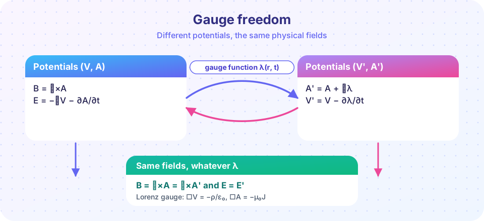
Because ∇·B = 0, B can be written as a curl: B = ∇×A. Put this in Faraday's law: ∇×(E + ∂A/∂t) = 0. A field with zero curl is a gradient, so E + ∂A/∂t = −∇V, i.e.
B = ∇×A
E = −∇V − ∂A/∂t
The two homogeneous equations (∇·B = 0 and Faraday) are now automatically true. Only Gauss and Ampere-Maxwell remain, and they become two coupled equations in V and A.
Gauge freedom
The potentials are not unique. Choose any smooth function λ(r, t) and set
A' = A + ∇λ, V' = V − ∂λ/∂t
Then ∇×A' = ∇×A because the curl of a gradient vanishes, and
E' = −∇V' − ∂A'/∂t = −∇V + ∇(∂λ/∂t) − ∂A/∂t − ∇(∂λ/∂t) = E.
The fields are untouched. This freedom is the gauge freedom, and it lets you pick the most convenient version.
Lorenz gauge
Imposing ∇·A = −μ₀ε₀ ∂V/∂t decouples the equations into two wave equations with the same operator:
□V = −ρ/ε₀, □A = −μ₀ J
Each component of A and V satisfies a wave equation with a source. In vacuum, the solutions travel at c. This is the form used for radiation in Chapter 7. The Coulomb gauge ∇·A = 0 gives ∇²V = −ρ/ε₀ (an instantaneous Poisson equation) plus a more complicated equation for A; it is popular in quantum optics and when only transverse radiation matters.
Worked example: a uniform magnetic field
For B = B₀ ẑ, one valid choice is A = (B₀/2)(−y, x, 0). Its curl is (0, 0, B₀). Another is the Landau choice A = (0, B₀x, 0). They differ by ∇λ with λ = B₀xy/2. Both give the same B.
Worked example: the vector potential of a solenoid
A long solenoid of radius R holds a uniform field B₀ inside and essentially none outside. By symmetry A circles the axis. Stokes' theorem makes this easy: ∮A·dl = ∫B·dA = Φ.
- Inside (
r < R):A (2π r) = B₀ π r², soA = B₀ r/2, the same form as the uniform-field choice above. - Outside (
r > R): the loop encloses the full fluxB₀ π R², soA = B₀ R²/(2r).
The surprise is the outside region. Here B = 0 but A = B₀R²/(2r) is not zero: for B₀ = 0.010 T and R = 1.0 mm it is 1.0×10⁻⁶ T·m at r = 5.0 mm. A vector potential that carries no field is perfectly legitimate, because its curl vanishes there. It is a pure gauge locally (A = ∇λ with λ ∝ φ), but you cannot remove it globally without a discontinuity, because the loop integral around the solenoid is the nonzero flux Φ.
The Aharonov-Bohm effect
In quantum mechanics a particle of charge q traveling along a path picks up a phase (q/ħ) ∫A·dl. Two beams that pass on opposite sides of the solenoid differ in phase by ΔΦ = qΦ/ħ, even though neither beam ever touches a magnetic field. Yakir Aharonov and David Bohm predicted this in 1959 (Ehrenberg and Siday had noted a version in 1949), and Akira Tonomura's group confirmed it with electron holography in 1986. The flux for B₀ = 0.010 T, R = 1.0 mm is Φ = 3.14×10⁻⁸ Wb, about 7.6 × 10⁶ flux quanta h/e = 4.14×10⁻¹⁵ Wb. Real experiments use tiny magnetized rings or whiskers carrying a fraction of one flux quantum, and the fringe pattern shifts by the fraction. The lesson: A is not directly measurable, but the loop integral ∮A·dl is, and it is gauge invariant.
Choosing a gauge
| Gauge | Condition | Equation for V | Best for |
|---|---|---|---|
| Lorenz | ∇·A = −μ₀ε₀ ∂V/∂t |
□V = −ρ/ε₀ |
Radiation, relativity: every equation is wave-like and Lorentz covariant |
| Coulomb | ∇·A = 0 |
∇²V = −ρ/ε₀ |
Static problems, quantum optics: V is the instantaneous Coulomb potential |
The Coulomb gauge looks as if it breaks causality, because V responds instantly to charge motion. It does not: the instant part is cancelled by a compensating term inside E = −∇V − ∂A/∂t, and the physical fields still propagate at c. The name "Lorenz gauge" honors Ludvig Lorenz (Denmark, 1867), not Hendrik Lorentz, though the two are often confused.
"The potentials are just math tricks; only E and B are real." In classical physics only E and B matter, but in quantum mechanics the Aharonov-Bohm effect shows that a particle's phase depends on A even where B = 0. What matters physically are gauge-invariant quantities such as ∮A·dl.
"V is the same V as in circuits." In electrostatics yes, but in dynamics E ≠ −∇V alone; you must add −∂A/∂t.
Try it
Press Run (or Ctrl + Enter) to see the result here.
Program input · what you'd type while the program runs
Type the answers before you press Run, one per line. Each time the program reads a line (with input()), it gets the next line from this box.
Press Run (or Ctrl + Enter) to see the result here.
Program input · what you'd type while the program runs
Type the answers before you press Run, one per line. Each time the program reads a line (with input()), it gets the next line from this box.
Press Run (or Ctrl + Enter) to see the result here.
Program input · what you'd type while the program runs
Type the answers before you press Run, one per line. Each time the program reads a line (with input()), it gets the next line from this box.
Check your understanding
Quick check · 6 questions
of 6 answered You scored / 6 · perfect!
-
1. Which pair of definitions is correct?
B = ∇×A guarantees ∇·B = 0, and E = −∇V − ∂A/∂t guarantees Faraday's law. -
2. Under the gauge transformation A' = A + ∇λ, what must V become?
V' = V − ∂λ/∂t cancels the extra −∂(∇λ)/∂t in E. -
3. Which gauge condition gives symmetric wave equations for V and A?
∇·A = −μ₀ε₀ ∂V/∂t gives □V = −ρ/ε₀ and □A = −μ₀J. -
4. Why is the gauge choice allowed?
All measurable fields and forces depend only on E and B, which are gauge-invariant. -
5. Outside a long solenoid of radius R carrying uniform field B₀ inside, the vector potential at distance r is
Stokes' theorem gives ∮A·dl = B₀πR², so A = B₀R²/(2r). Its curl is zero but its loop integral is the enclosed flux. -
6. The Aharonov-Bohm effect shows that
The interference shift depends on the enclosed flux, a gauge-invariant loop integral of A.
Summary
B = ∇×AandE = −∇V − ∂A/∂tsolve two Maxwell equations automatically.- Gauge transformations
A → A + ∇λ,V → V − ∂λ/∂tleave E and B unchanged. - Lorenz gauge:
□V = −ρ/ε₀,□A = −μ₀J. - Gauge-invariant combinations are the physical ones.
- Outside a solenoid
A = B₀R²/(2r)is nonzero thoughB = 0; the Aharonov-Bohm phaseqΦ/ħis the evidence that∮A·dlis physical. - The Coulomb gauge suits statics, the Lorenz gauge suits waves; both give the same E and B.
Next: Chapter review
Track your progress
Create a free account to tick off lessons and pick up where you left off on any device.
of Electrodynamics lessons completed