


















Lesson 3 of 49 · Getting Started
The electric field and superposition
Learn the electric field as force per charge, draw field lines, add fields of many charges, and compute fields of rods, rings and disks with worked examples and code.
Coulomb's law tells you the force between two charges. But if a thousand charges are around, you would have to recompute everything each time you place a new test charge. The electric field fixes this. Instead of asking "what force would a charge feel here?", you ask "what does the space around these charges look like?" and record the answer at every point once. The field is the stage on which all of electrodynamics is played.
What you will learn
- The definition of the electric field as force per unit test charge, and its units.
- How to draw and read field lines, and what they can and cannot tell you.
- How to compute fields of point charges, rods, rings and disks by superposition.
- Why symmetry arguments save so much work.
Key terms
- Electric field E: the force per unit charge,
E = F / q, measured in N/C (identical to V/m). - Test charge: a small charge used to probe a field without disturbing the sources.
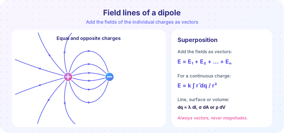
- Field line: a curve whose tangent is the direction of E; it starts on positive charge and ends on negative.
- Charge density: charge per length (λ), area (σ) or volume (ρ).
- Dipole: a pair of equal and opposite charges a small distance apart.
From force to field
Place a small test charge q at a point and measure the force F on it. The ratio
E = lim (F / q) as q → 0
does not depend on q. It is a property of the sources only. The limit is a reminder that the test charge must be small enough not to move the sources. Once you know E everywhere, the force on any charge is just F = qE.
For a single point charge Q at the origin, Coulomb's law gives
E(r) = k Q r̂ / r²
pointing away from positive Q and toward negative Q. Because the 1/r² law is the same for every charge, the field of many point charges is the vector sum
E(r) = Σ k qᵢ r̂ᵢ / rᵢ² where rᵢ is the vector from charge i to the field point.
Field lines
Field lines are drawn so that the tangent at each point gives the direction of E, and the density of lines indicates the strength. Three rules follow from the structure of the field:
- Lines start on positive charges and end on negative charges (or run off to infinity).
- Lines never cross, because E has one direction at each point.
- Lines are densest where the field is strongest: near the charges, between the closely spaced charges of a dipole.
Field lines are a picture, not a physical thing. A line has no thickness or tension, and the number of lines drawn is arbitrary. But for a 3D field the rule "the number of lines through a surface is proportional to the flux" is exactly Gauss's law, which comes next chapter.
Continuous charge distributions
For a continuous distribution, chop the charge into small pieces dq, find each contribution dE = k dq r̂ / r², and integrate:
E = k ∫ r̂ dq / r²
The element dq depends on the geometry:
| Distribution | Density | dq |
|---|---|---|
| Line | λ (C/m) | λ dl |
| Surface | σ (C/m²) | σ dA |
| Volume | ρ (C/m³) | ρ dV |
Worked example 1: a finite rod
A rod of length L carries uniform charge density λ along the x axis, centered at the origin. Find E at a point a distance s from the rod on its perpendicular bisector.
Symmetry says the components along the rod cancel in pairs, so only the component perpendicular to the rod survives. A piece at position x has dq = λ dx, distance √(s² + x²) and perpendicular component s / √(s² + x²):
E = k λ ∫ s dx / (s² + x²)^{3/2} from −L/2 to L/2
The integral is x / (s √(s² + x²)), so
E = k λ L / (s √(s² + L²/4))
Check the limit L → ∞: the square root becomes L/2, giving E = 2kλ / s, the field of an infinite line. For λ = 1 nC/m and s = 10 cm, an infinite line gives about 180 N/C, a 20 cm rod about 127 N/C.
Worked example 2: a ring and a disk on the axis
For a ring of radius R and total charge Q, each element contributes a component along the axis z / √(z² + R²); the perpendicular components cancel around the ring:
E_z = k Q z / (z² + R²)^{3/2}
Far away (z ≫ R) this becomes kQ / z², the point charge result, as it should. Stack rings from radius 0 to R, with charge σ 2π a da each, to get a disk of surface density σ:
E_z = (σ / 2ε₀) [1 − z / √(z² + R²)]
As R → ∞ the bracket goes to 1 and E = σ / (2ε₀), the famous field of an infinite plane, constant and independent of distance.
The dipole
Two charges +q and −q separated by a small distance d make a dipole with moment p = q d (pointing from − to +). Far away the field falls off as 1/r³: on the axis, E = 2kp / z³; on the perpendicular bisector, E = kp / r³ pointing opposite to p. Atoms and molecules are dipoles, which is why this will return in Chapter 3.
Common misconceptions
- "Field lines are the paths charges follow." Only for a particle released from rest and moving slowly with no inertia. Generally a charge has momentum and does not follow a line.
- "A field exists only if a test charge is there." The field is there regardless; the test charge only reveals it.
- "The field at a point is zero if the field lines do not pass through it." Lines are a finite sample; the field is defined everywhere.
- "Add the magnitudes of the individual fields." Fields are vectors. Equal fields of opposite direction cancel.
Try it
The first demonstration is an interactive field map of two charges: move the sliders and watch the arrows. The second checks the rod formula against a numeric integral, and the third shows how a charged disk approaches the infinite-plane field.
Press Run (or Ctrl + Enter) to see the result here.
Program input · what you'd type while the program runs
Type the answers before you press Run, one per line. Each time the program reads a line (with input()), it gets the next line from this box.
Press Run (or Ctrl + Enter) to see the result here.
Program input · what you'd type while the program runs
Type the answers before you press Run, one per line. Each time the program reads a line (with input()), it gets the next line from this box.
Check your understanding
Quick check · 5 questions
of 5 answered You scored / 5 · perfect!
-
1. A charge of 2.0 μC feels a force of 0.05 N. What is the electric field at its position?
E = F/q = 0.05 / 2.0e-6 = 2.5e4 N/C. -
2. Which statement about electric field lines is true?
Lines do not cross (the field has one direction at each point), and they begin and end on charges. -
3. What is the field of a very long uniformly charged line at distance s?
Integrating the contributions of the line gives E = 2kλ/s, which falls off as 1/s, not 1/s². -
4. Why does the component of E along the axis of a ring survive while perpendicular components cancel?
Each element has a partner on the opposite side whose perpendicular component is equal and opposite. -
5. A dipole's field far away drops as
The two opposite charges nearly cancel; the remaining field falls as 1/r³.
Summary
E = F / qis the force per unit test charge; the force on any charge isF = qE.- The field of a point charge is
kQ r̂ / r²; fields of many sources add as vectors (superposition). - Field lines start on positive charges, end on negative ones and never cross.
- Continuous charge:
E = k ∫ r̂ dq / r²; use symmetry to cancel components first. - Key results: infinite line
2kλ/s, ring on axiskQz/(z²+R²)^{3/2}, infinite planeσ/2ε₀, dipole~ 1/r³.
Track your progress
Create a free account to tick off lessons and pick up where you left off on any device.
of Electrodynamics lessons completed