


















Lesson 37 of 49 · Radiation and Antennas
Antennas: half-wave dipole, gain and the Friis equation
From the short dipole to the half-wave dipole: radiation patterns, radiation resistance, directivity and gain, and a radio link budget with the Friis equation.
A real antenna is larger than the idealized point dipole, and the current along it is not uniform. The half-wave dipole, a straight wire about half a wavelength long fed at its center, is the reference design of radio engineering. Its pattern, impedance and gain can be derived by adding up the radiation from tiny current elements, and its numbers appear in every radio handbook.
What you will learn
- Compare the short dipole with the half-wave dipole.
- Use radiation resistance, directivity and gain.
- Compute a free-space link with the Friis transmission equation.
- Relate antenna length to wavelength.
Key terms
Radiation resistance R_rad: the resistance that would dissipate the radiated power, P = ½ I₀² R_rad. Directivity D: peak radiation intensity divided by its average over all directions. Gain G = η D, with η the efficiency. dBi: gain in decibels over an isotropic radiator. Effective aperture A_e = Gλ²/(4π).
The short dipole
For a dipole of length ℓ ≪ λ with current tapering linearly to zero at the ends, the radiation resistance is
R_rad = 20 π² (ℓ/λ)²
For ℓ = λ/10 this is only 1.97 Ω, so a short antenna is a poor radiator and ohmic losses and mismatch dominate. The pattern is sin²θ with directivity D = 1.5 (1.76 dBi).
The half-wave dipole
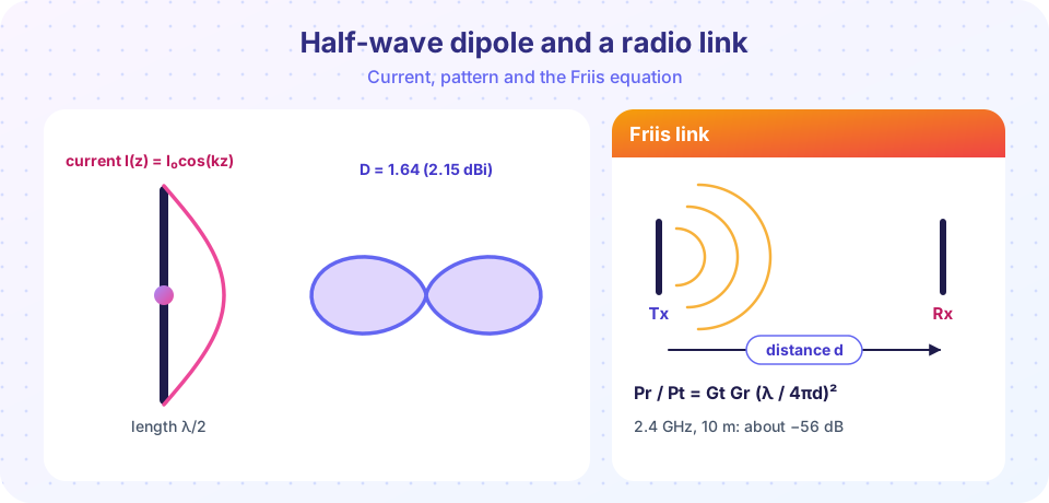
With ℓ = λ/2 the current is approximately I(z) = I₀ cos(kz), zero at the ends and maximum at the feed point. Adding up the radiation from each element gives the field pattern
F(θ) = cos((π/2) cos θ) / sin θ
and a power pattern F².
Where the pattern comes from
Cut the wire into tiny elements dz, each a short dipole carrying I₀ cos(kz). In the far zone the elements all point the same way, so their fields add with different phases: an element at height z is closer to the observer by z cosθ, so its wave arrives early by a phase k z cosθ. The total field is proportional to
sinθ ∫ cos(kz) e^{j k z cosθ} dz   (z from −λ/4 to +λ/4)
 = (2/k) cos((π/2) cosθ) / sinθ
The sinθ is the single-element pattern; the integral is the array factor of the wire. At θ = 90° all elements add in phase, so that direction is the maximum; along the axis the factor cos((π/2)cosθ) is zero, which kills the radiation there. Squaring gives the power pattern, and integrating it over the sphere gives the total power, from which R_rad = 2P/I₀² follows. The lesson's TryIt does this integral numerically and lands on 73.1 Ω. The result needs a sine-integral (Si, Ci) in closed form, which is why handbooks quote 73.1 rather than a neat expression.
For the numbers:
| Quantity | Half-wave dipole |
|---|---|
| Radiation resistance | ≈ 73.1 Ω |
| Directivity | 1.64 (2.15 dBi) |
| Half-power beamwidth | 78° in the plane containing the axis |
| Pattern | figure-eight, null on the axis |
A practical dipole is about 5% shorter than λ/2 (end effects) to make the reactance zero. At 100 MHz, λ = 3.0 m so each arm is about 0.71 m in total length 1.43 m. Since 73 Ω is close to 75 Ω coaxial cable, matching is easy.
A quarter-wave monopole over a ground plane is half of a dipole: radiation resistance about 36.5 Ω, directivity 3.28 (5.15 dBi) over the half-space above ground.
Gain, aperture and the Friis equation
A receiving antenna of gain G_r intercepts power from a plane wave of intensity I equal to I A_e with A_e = G_r λ²/(4π). A transmitter of power P_t and gain G_t produces I = P_t G_t/(4π d²) at distance d, so
P_r / P_t = G_t G_r (λ / (4π d))²
This is the Friis transmission equation (free space, matched, aligned, polarization matched). The factor (λ/4πd)² is called free-space path loss and grows with frequency for fixed antenna gains because the aperture shrinks.
Worked example: a Wi-Fi link
f = 2.4 GHz, so λ = 0.125 m. Two half-wave dipoles with G = 1.64 at d = 10 m:
(λ/(4πd))² = (0.125 / 125.7)² = 9.9 × 10⁻⁷
P_r/P_t = 1.64² × 9.9 × 10⁻⁷ = 2.7 × 10⁻⁶  →  −55.8 dB
With P_t = 100 mW (20 dBm) the received power is about −35.8 dBm, or 0.27 µW. Real indoor links lose more to walls and multipath.
Decibels in one minute
Link budgets are added, not multiplied, because engineers use decibels: X_dB = 10 log₁₀ X. A factor of 2 in power is +3 dB, a factor of 10 is +10 dB, a factor of 4 is +6 dB. Absolute power is quoted in dBm (decibels above 1 mW), so 100 mW is +20 dBm. Friis in decibels reads P_r(dBm) = P_t(dBm) + G_t(dBi) + G_r(dBi) − L_path(dB), with L_path = 20 log₁₀(4πd/λ). For the Wi-Fi example L_path = 20 log₁₀(125.7/0.125) = 60.0 dB, G_t + G_r = 2 × 2.15 = 4.3 dB, so P_r = 20 + 4.3 − 60.0 = −35.7 dBm, the same result as before to rounding.
Worked example: an FM radio link
A station radiates P_t = 10 kW at 100 MHz (λ = 3.0 m) and you listen 10 km away, both antennas being half-wave dipoles (G = 1.64):
(λ/(4πd))² = (3.0 / 125 664)² = 5.7 × 10⁻¹⁰
P_r = 10⁴ W × 1.64² × 5.7 × 10⁻¹⁰ ≈ 1.5 × 10⁻⁵ W  (15 µW, −18 dBm)
That is a strong signal; a car radio can pick up stations at a millionth of this power. The effective aperture of the receiving dipole is A_e = Gλ²/4π = 1.64 × 9/12.57 ≈ 1.17 m²: the dipole "collects" the power that crosses an area bigger than itself. At 2.4 GHz the same gain gives only A_e ≈ 2 × 10⁻³ m², which is why a Wi-Fi link at the same distance is so much weaker even though nothing about physics has changed but the wavelength.
Matching the antenna to the cable
An antenna feeds power through a transmission line of characteristic impedance Z₀ (50 Ω is the usual choice in radio equipment, 75 Ω in video). A load Z_L reflects a fraction Γ = (Z_L − Z₀)/(Z_L + Z₀) of the voltage. A resonant half-wave dipole (Z_L ≈ 73 Ω) on 50 Ω cable has Γ = 23/123 = 0.19, the standing-wave ratio is VSWR = (1 + Γ)/(1 − Γ) = 1.46, and the reflected power is Γ² = 3.5%, a mismatch loss of just 0.16 dB. For a short dipole with R_rad = 2 Ω and a large capacitive reactance, Γ is close to 1 and most of the power bounces back, so a matching network is essential.
Heinrich Hertz's 1887 transmitter was a dipole with metal spheres at the ends, and Marconi's first transatlantic signal (1901) used a very long wire. Modern engineers describe antennas by pattern, impedance and gain, the three numbers in this lesson. The transmission formula in this lesson was published by Harald Friis in 1946.
"Higher gain means the antenna creates more power." Gain is redistribution of the same power into some directions, at the expense of others.
"An antenna of any length works equally well." An antenna much shorter than λ/2 is a poor radiator and has a large reactance.
"A dipole radiates equally in all directions." An isotropic radiator is only a reference; the half-wave dipole has a figure-eight with a null on its axis.
Try it
Press Run (or Ctrl + Enter) to see the result here.
Program input · what you'd type while the program runs
Type the answers before you press Run, one per line. Each time the program reads a line (with input()), it gets the next line from this box.
Press Run (or Ctrl + Enter) to see the result here.
Program input · what you'd type while the program runs
Type the answers before you press Run, one per line. Each time the program reads a line (with input()), it gets the next line from this box.
Press Run (or Ctrl + Enter) to see the result here.
Program input · what you'd type while the program runs
Type the answers before you press Run, one per line. Each time the program reads a line (with input()), it gets the next line from this box.
Check your understanding
Quick check · 7 questions
of 7 answered You scored / 7 · perfect!
-
1. A half-wave dipole is designed for 300 MHz. Its ideal length is
λ = c/f = 1.0 m, so λ/2 = 0.5 m (a bit shorter in practice). -
2. The radiation resistance of a half-wave dipole is about
≈ 73 Ω, close to 75 Ω coaxial cable. -
3. Friis's equation says received power falls with distance as
P_r/P_t ∝ (λ/4πd)². -
4. If the frequency doubles with both antenna gains fixed, free-space received power changes by
λ halves and the factor (λ/4πd)² quarters, so power drops to a quarter. -
5. Which pattern is zero along the antenna axis?
The figure-eight pattern of a dipole has nulls along the wire. -
6. A 73 Ω dipole is connected to a 50 Ω cable. About what fraction of the power is reflected?
Γ = 23/123 = 0.19 is the voltage reflection; the power fraction is Γ² ≈ 0.035. -
7. Why does the received power in a Friis link drop when the frequency rises, with fixed antenna gains?
A fixed-gain antenna collects over an area proportional to λ², so shorter waves are captured over a smaller area.
Summary
- Short dipole:
R_rad = 20π²(ℓ/λ)²,D = 1.5; half-wave dipole:R_rad ≈ 73 Ω,D = 1.64. - Half-wave pattern
[cos((π/2)cosθ)/sinθ]², null on the axis. - Effective aperture
A_e = Gλ²/4π; Friis:P_r/P_t = G_tG_r(λ/4πd)².
Next: Chapter review
Track your progress
Create a free account to tick off lessons and pick up where you left off on any device.
of Electrodynamics lessons completed