


















Lesson 43 of 49 · Projects and Practice
Chapter overview: projects and practice
Put electrodynamics to work with two simulation projects, ten practice problems, a glossary, a cheat sheet and a guide to further study.
You now have the whole structure of classical electrodynamics: fields from charges, Maxwell's equations, waves, radiation and relativity. Understanding comes from using it. This last chapter turns the theory into running code and numerical practice, then gives you the tools to review and continue.
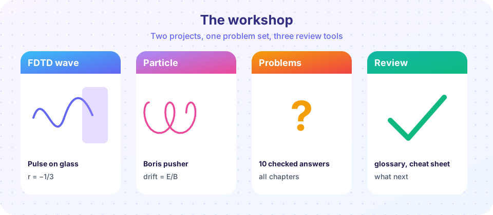
What you will build and review
| Lesson | What you do | Skills used |
|---|---|---|
| Project: 1D FDTD simulation | Simulate a pulse hitting a dielectric and measure the reflection | Maxwell's curl equations, boundary behavior |
| Project: charged particle in fields | Track an electron with the Boris method and verify drift | Lorentz force, cyclotron motion |
| Practice problems | Ten calculations with checked answers | All chapters |
| Glossary | Look up terms and test yourself | Vocabulary |
| Cheat sheet | One page of formulas and constants | Revision |
| Further study | Where to go next | Planning |
How to use the projects. Run each TryIt, then change one parameter at a time (the permittivity, the time step, the magnetic field) and predict the result before pressing Run. Disagreements between prediction and result are where the learning happens.
Press Run (or Ctrl + Enter) to see the result here.
Program input · what you'd type while the program runs
Type the answers before you press Run, one per line. Each time the program reads a line (with input()), it gets the next line from this box.
How a computational physicist works
A simulation is only worth believing after it has passed tests. Professionals follow a loop, and both projects follow it.
- Start from a case with a known answer. In the FDTD project it is the Fresnel reflection
r = (1 − n)/(1 + n); in the particle project, the cyclotron frequency and theE×Bdrift. - Check invariants. Energy must balance (
R + T = 1), the speed must not change in a pure magnetic field, andc²B² − E²must be the same in every frame. - Vary the numerics. Halve the time step or double the resolution. A result that moves a lot is not converged.
- Break it on purpose. Choose
S > 1, or an Euler step for the magnetic force, and watch what failure looks like. You will recognize it later. - Only then explore. Change the physics and trust the answer.
Real research follows the same pattern. Kane Yee's 1966 paper introduced the grid used in the first project; the Boris scheme of about 1970 is still the default in plasma codes; both survive because they respect a structure of the equations (staggered curls, or exact rotation) rather than being merely small-step approximations.
What good results look like
| Project | Check | Expected value |
|---|---|---|
| FDTD | reflection amplitude r for n = 2 |
−0.333 (simulation gives about −0.334) |
| FDTD | transmission amplitude t |
0.667 |
| FDTD | thin film R at the quarter-wave frequency |
0.36 |
| Particle | electron f_c in 1 mT |
28.0 MHz |
| Particle | drift speed for E = 100 V/m, B = 1 mT |
10⁵ m/s, any species |
| Particle | gyroradius at 2 × 10⁵ m/s in 1 mT |
1.14 mm |
If your output differs from these by more than a percent, look for a unit error first (millitesla versus tesla is the usual culprit), then a time step that is too large.
"The simulation says so, so it is true." A program only solves the equations you gave it with the errors you allowed. "More digits mean more accuracy." Printing eight digits of a number that is only converged to two just prints noise. "Hard to code means advanced physics." The most powerful ideas here, the staggered grid and the rotation step, are four lines each.
Scales to keep in mind
Before coding, ask what size and speed matter. A 10 MHz wave has a wavelength of 30 m, a visible light wave 500 nm. A grid needs about 20 cells per wavelength, so a 1D grid for a 1 GHz wave (λ = 0.30 m) needs a cell of about 1.5 cm. The Courant condition then fixes the time step at Δx/c ≈ 50 ps, so one nanosecond of physical time takes only 20 steps. A gyrating electron in 1 mT has a period of 35.7 ns, and 100 steps per period means Δt = 0.36 ns.
Press Run (or Ctrl + Enter) to see the result here.
Program input · what you'd type while the program runs
Type the answers before you press Run, one per line. Each time the program reads a line (with input()), it gets the next line from this box.
Check your understanding
Quick check · 5 questions
of 5 answered You scored / 5 · perfect!
-
1. Why change one parameter at a time in a simulation?
Changing a single variable isolates its effect and lets you test your predictions. -
2. Which constant gives the vacuum impedance when combined as √(μ₀/ε₀)?
Z₀ = √(μ₀/ε₀) ≈ 376.7 Ω. -
3. What should you do before running a modified simulation?
A prediction turns running code into a test of your understanding. -
4. Why start a new simulation from a case with a known analytic answer?
A match with a trusted result shows the code solves the equations correctly. -
5. A 1 GHz wave has a wavelength of about 0.30 m. With 20 cells per wavelength, the cell size is about
0.30 m / 20 = 0.015 m = 1.5 cm.
Summary
- The projects use the same equations you derived, discretized or integrated numerically.
- The practice problems have checked numerical answers.
- The glossary, cheat sheet and further-study guide support revision and next steps.
Track your progress
Create a free account to tick off lessons and pick up where you left off on any device.
of Electrodynamics lessons completed