


















Lesson 44 of 49 · Projects and Practice
Project: a 1D FDTD simulation of a pulse hitting glass
Build a one-dimensional finite-difference time-domain solver for Maxwell's curl equations, send a pulse into a dielectric slab and measure the reflection coefficient.
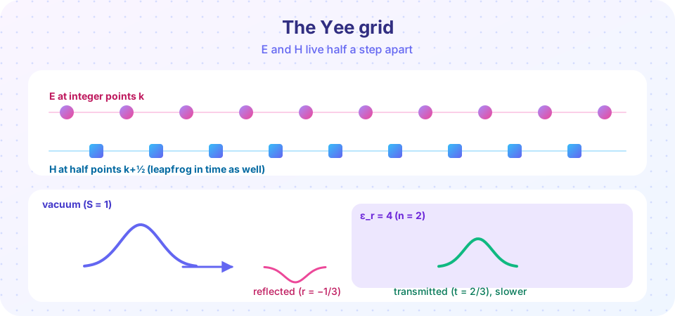
The finite-difference time-domain (FDTD) method, introduced by Kane Yee in 1966, marches Maxwell's two curl equations forward in time on a grid. It needs no matrix inversion, it handles any material, and 40 lines of Python are enough for a working one-dimensional version. In this project you launch a pulse, let it hit a dielectric half-space with n = 2, and compare the measured reflection with the Fresnel prediction from Chapter 6.
What you will learn
- Discretize the 1D curl equations on a Yee grid.
- Choose a stable time step (the Courant condition).
- Add a dielectric region and a pulse source.
- Extract the reflection coefficient from the simulation and compare it with theory.
Key terms
Yee grid: E and H stored half a cell and half a time step apart. Courant number S = c Δt/Δx; stability in 1D needs S ≤ 1. Leapfrog: alternately updating E and H. Soft source: a source added to the field instead of overwriting it. Absorbing boundary: a boundary condition that lets waves leave without reflecting.
The equations
For a wave traveling along z with E = E_x(z, t) x̂ and H = H_y(z, t) ŷ, Maxwell's curl equations reduce to
∂H_y/∂t = (1/μ₀) ∂E_x/∂z
∂E_x/∂t = (1/ε) ∂H_y/∂z       (ε = ε₀ ε_r)
Use normalized units in which c = 1, Δx = 1 and a quantity E scaled so that μ₀ = ε₀ = 1. On the Yee grid the updates are
H[k] += S (E[k+1] − E[k])
E[k] += S (H[k] − H[k−1]) / ε_r[k]
For S = 1 and ε_r = 1 a pulse moves exactly one cell per step with no numerical dispersion. In a dielectric with ε_r = 4 (index n = 2) the local Courant number is S/n = 0.5, the wave speed halves, and the wavelength halves.
The experiment
We run the simulation twice, with and without the slab, and subtract: the difference is the reflected pulse only. The ratio of its peak to the incident peak is the amplitude reflection coefficient. Fresnel predicts r = (1 − 2)/(1 + 2) = −1/3: the reflected pulse is inverted, with one third of the amplitude and R = 1/9 of the power.
Press Run (or Ctrl + Enter) to see the result here.
Program input · what you'd type while the program runs
Type the answers before you press Run, one per line. Each time the program reads a line (with input()), it gets the next line from this box.
From the curl equations to the update rules
Replace each derivative by a centered difference. For the magnetic field, evaluated half a time step later and half a cell to the right of an E point,
(H[k]^(n+½) − H[k]^(n−½))/Δt = (1/μ₀) (E[k+1]^n − E[k]^n)/Δx
Solving for the new H gives H[k] += (Δt/μ₀Δx)(E[k+1] − E[k]). The electric equation is the same with the roles swapped and a factor 1/ε. Because each difference is centered on the point being updated, the error is second order in Δx and Δt. The staggering is also what makes the scheme explicit: the new H needs only old E and the new E needs only the new H, so each step is two vector additions.
The normalized constants come from one choice. Define S = cΔt/Δx. Scaling H by the impedance Z₀ = √(μ₀/ε₀) ≈ 377 Ω makes both updates look the same, with the factor S in front. We took S = 1. In a region with relative permittivity ε_r the factor becomes S/ε_r in the E update, so the grid has the same Δx but the pulse crosses a cell in n steps instead of one.
Why S ≤ 1: stability and dispersion
Information travels one cell per step at most in this scheme, because each update touches only neighbors. If the physical signal moves faster than the grid can carry it (S > 1), the numerical solution cannot follow, and errors grow exponentially. This is the one-dimensional Courant-Friedrichs-Lewy condition. In 2D it tightens to S ≤ 1/√2 and in 3D to S ≤ 1/√3.
For S < 1 the scheme is stable but slightly dispersive. Substituting a traveling wave into the updates gives the numerical dispersion relation
sin(ω Δt/2) = S sin(k Δx/2)
and the numerical phase speed follows. For S = 1 it equals c exactly at every wavelength (a magic property of 1D). For S = 0.5 and 20 cells per wavelength the speed is 0.997 c, and with 10 cells it is 0.988 c. The rule of thumb is at least 10, and preferably 20, cells per shortest wavelength. Inside the dielectric the wavelength is n times shorter, so the effective resolution there is lower and the local Courant number is S/n.
Press Run (or Ctrl + Enter) to see the result here.
Program input · what you'd type while the program runs
Type the answers before you press Run, one per line. Each time the program reads a line (with input()), it gets the next line from this box.
The first table reproduces the numbers above. The second part kicks the grid once and watches it: for S ≤ 1 the field stays bounded, while S = 1.05 grows by more than a hundred orders of magnitude in 400 steps.
Worked check: what should the pulse do?
Before trusting a simulation, predict three numbers by hand for n = 2. The amplitude reflection coefficient is r = (1 − 2)/(1 + 2) = −1/3. The transmission coefficient is t = 2/(1 + 2) = 2/3. Energy must balance: the reflected power fraction is R = 1/9 = 0.111, so the transmitted fraction is 8/9. Check it with the fields: the transmitted power per area is n t² = 2 × 4/9 = 8/9 of the incident, because the intensity scales with the index times the squared amplitude. The numbers add up to 1/9 + 8/9 = 1. If your code printed a t of 0.667 and an r of −0.333 but your energy sum was 1.2, you would know something was wrong.
Why is r negative? At the boundary the tangential E must be continuous, 1 + r = t, and so must the tangential H, (1 − r) = n t. Solving gives r = (1 − n)/(1 + n). A wave going into a slower medium therefore reflects with the opposite sign, just like a pulse on a light rope meeting a heavy one.
Extension: a thin film and its colors
Make the slab only d = 40 cells wide, with vacuum on both sides. Two reflections now interfere: one from the front face and one from the back. In a thin film of index n the round trip phase is 2δ with δ = 2π n d f (frequency f in cycles per step, c = 1 cell per step). The film's reflectance is
r = r₁₂ (1 − e^(2iδ)) / (1 − r₁₂² e^(2iδ)), R = |r|²
with r₁₂ = (1 − n)/(1 + n). When n d = λ/4 the two reflections add and R reaches its maximum (2r₁₂/(1 + r₁₂²))² = 0.36. When n d = λ/2 they cancel and R = 0. This is why soap bubbles and oil slicks show colors and why anti-reflection coatings work. We can recover the whole curve from one pulse: its spectrum covers many frequencies, so the Fourier transform of the reflected pulse divided by that of the incident one gives R(f).
Press Run (or Ctrl + Enter) to see the result here.
Program input · what you'd type while the program runs
Type the answers before you press Run, one per line. Each time the program reads a line (with input()), it gets the next line from this box.
The simulated and theoretical columns agree to within a few percent: the largest reflectance sits near the quarter-wave frequency (about 0.0031), and it drops to nearly zero at the half-wave frequency (0.00625), where n d = λ/2. The remaining small differences come from numerical dispersion and the finite pulse bandwidth.
Make an anti-reflection coating. Put a film of index √2 ≈ 1.41 (the geometric mean of 1 and 2) in front of the n = 2 half-space, with thickness λ/(4n). Both reflections now have the same size and opposite signs, so the reflection at that wavelength vanishes. Try it by setting eps_r to 2.0 for the film cells and 4.0 beyond them.
Try changing things
- Index. Set
slab[450:] = 9.0(n = 3). Theory predictsr = −0.5. - Time step. Halve the source width; a narrow pulse makes the dispersion error visible at
S < 1. - Thin film. Make the slab only 40 cells wide; the two reflections will interfere. Measure how the total reflection depends on the slab thickness compared with the wavelength in the film.
"If the numbers are close, the code is correct." A reflection of −0.33 could hide an error elsewhere (like the wrong energy). Always check a second quantity, such as the transmitted amplitude t = 2/(1+n) = 0.667.
"Any time step works." For S > 1 the scheme is unstable and the values grow without bound.
"The boundary condition is a detail." An unabsorbed reflection from the grid edge looks exactly like a physical echo. Here we avoid it by making the grid long enough that edges are not reached during the run.
Try it
Press Run (or Ctrl + Enter) to see the result here.
Program input · what you'd type while the program runs
Type the answers before you press Run, one per line. Each time the program reads a line (with input()), it gets the next line from this box.
Check your understanding
Quick check · 6 questions
of 6 answered You scored / 6 · perfect!
-
1. In the 1D Yee scheme, which statement is true?
Staggering gives second-order accuracy and a simple explicit update. -
2. What reflection coefficient does theory predict for a pulse going from vacuum into n = 3?
r = (1 − 3)/(1 + 3) = −0.5. -
3. What goes wrong if the Courant number is above 1 in 1D?
The numerical signal cannot keep up with the physical one, so errors grow exponentially. -
4. How is the reflected pulse isolated in the project?
Without the slab there is no reflection, so the difference contains only the reflected wave. -
5. Why is r negative for a pulse entering a medium with a higher index?
Continuity gives 1 + r = t and 1 − r = n t, so r = (1 − n)/(1 + n), which is negative for n > 1. -
6. In the thin-film experiment, what is the reflectance when the optical thickness n d equals half a wavelength?
At half-wave thickness the round-trip phase is 2π, and the two reflections have opposite sign, so they cancel.
Summary
- FDTD updates E and H alternately on a staggered grid; stability needs
S ≤ 1. - A dielectric lowers the speed by
nand produces a reflectionr = (1 − n)/(1 + n). - Comparing a vacuum and a slab run isolates the reflected pulse.
Next: Project: a charged particle in electric and magnetic fields
Track your progress
Create a free account to tick off lessons and pick up where you left off on any device.
of Electrodynamics lessons completed