


















Lesson 17 of 49 · Magnetostatics
Chapter 4 overview: magnetostatics
Preview magnetism from steady currents: the Lorentz force, the Biot-Savart law, Ampère's law, the vector potential and magnetic materials, with the two equations of magnetostatics.
In 1820 Hans Christian Ørsted noticed that a compass needle twitched when a current started in a nearby wire. Within weeks André-Marie Ampère showed that parallel wires push and pull on each other. Magnetism, long known from lodestones, turned out to be a consequence of moving electric charge. This chapter treats the simplest case: steady currents that do not change in time. Then the magnetic field B is a fixed pattern in space, and almost everything about it can be found with the same tools as electrostatics: a force law, a source law, a symmetry-based shortcut and a potential.
What you will learn
- What steady current means and how it is described by the current density J.
- The two equations of magnetostatics,
∇·B = 0and∇×B = μ₀J. - How the lessons of this chapter fit together, and how magnetic work differs from electric work.
Key terms
- Magnetic field B: the field that exerts a force on moving charges; unit tesla (T).
- Current I: charge crossing a surface per second; unit ampere (A).
- Current density J: current per unit area, a vector in A/m².
- Steady current: constant in time, so charge does not pile up anywhere:
∇·J = 0. - Magnetic monopole: a hypothetical isolated magnetic pole; none has ever been found.
The big picture
Force
Sources
Structure
Matter
Parallel to the electric chapter, with a twist
The five lessons
- The Lorentz force: how a magnetic field pushes on moving charges and currents, circular and helical motion, and the cyclotron.
- The Biot–Savart law: the field of any steady current by adding the contribution of each element, with loops and wires.
- Ampère's law: the symmetry shortcut for B, with wires, solenoids and toroids.
- The vector potential and magnetic materials:
B = ∇×A, magnetization, the H field and ferromagnetism. - Chapter 4 review: the poster and quiz.
Steady currents
A current is a flow of charge. If a surface is crossed by a charge dq in time dt, I = dq/dt. In a wire with n free electrons per unit volume, each of charge −e and average drift velocity v_d, the current density is J = n q v_d (a vector in A/m²) and the current through area A is I = J A. The drift speed is tiny: for 1 A in a 1 mm² copper wire it is only about 0.07 mm/s, yet the whole wire carries current at once because the electrons are already everywhere.
"Steady" means that the charge density does not change in time anywhere. The conservation of charge says ∂ρ/∂t = −∇·J, so steady currents obey ∇·J = 0: current lines close on themselves, with no sources or sinks.
The two equations of magnetostatics
Parallel to Gauss's law and the zero curl of E:
∇·B = 0 (no magnetic charges: field lines never begin or end)
∇×B = μ₀ J (Ampère's law: currents curl the field)
with μ₀ = 1.2566 × 10⁻⁶ N/A². The first says magnetic field lines close on themselves. The second says that currents produce circulation. In the whole chapter you will keep returning to a contrast: electric field lines start on charges; magnetic field lines go around currents.
Common misconceptions
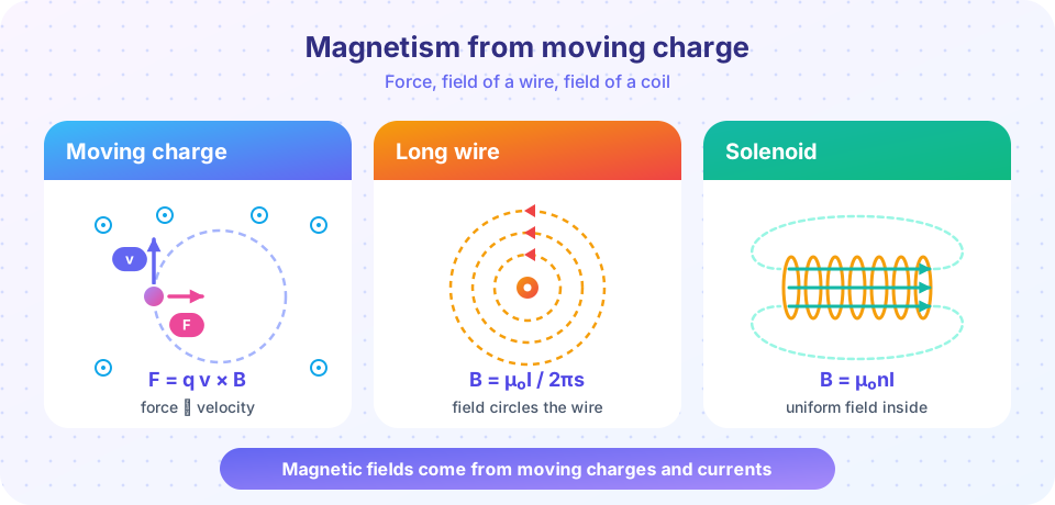
- "Magnetic fields come from magnets only." Magnets are made of moving charges: spinning electrons and orbital motion. Every magnetic field is generated by moving charge (or changing electric fields, Chapter 5).
- "Magnetic force can accelerate a charge." It changes its direction but never its speed, because
F ⊥ vmeans no work is done. - "Cutting a magnet makes a separate north and south pole." Each piece is a smaller magnet with two poles: no monopole exists.
Try it
The first example computes the field of a long wire and compares it with the Earth's field. The second computes the drift velocity of electrons.
Press Run (or Ctrl + Enter) to see the result here.
Program input · what you'd type while the program runs
Type the answers before you press Run, one per line. Each time the program reads a line (with input()), it gets the next line from this box.
Press Run (or Ctrl + Enter) to see the result here.
Program input · what you'd type while the program runs
Type the answers before you press Run, one per line. Each time the program reads a line (with input()), it gets the next line from this box.
Check your understanding
Quick check · 4 questions
of 4 answered You scored / 4 · perfect!
-
1. Which pair of equations describes magnetostatics?
No magnetic charges, and currents curl the field. -
2. A charge moves with velocity v in a magnetic field B. The magnetic force on it
F = qv×B is perpendicular to v, so F·v = 0. -
3. Why are steady currents described by ∇·J = 0?
Conservation of charge ∂ρ/∂t = −∇·J with ∂ρ/∂t = 0. -
4. Electrons drift in a wire at about
Typical drift speeds are ~10⁻⁴ m/s; the signal still moves very fast because the field propagates.
Summary
- Magnetic fields come from moving charges; steady currents satisfy
∇·J = 0. - Magnetostatics:
∇·B = 0and∇×B = μ₀J. - The magnetic force
qv×Bdoes no work; electrons drift slowly in wires. - The chapter develops the force law, the Biot–Savart law, Ampère's law, the vector potential and magnetic matter.
Next: The Lorentz force
Track your progress
Create a free account to tick off lessons and pick up where you left off on any device.
of Electrodynamics lessons completed