


















Lesson 36 of 42 · Food Security and Economics
Farm Economics and Markets
Learn to build a farm budget, calculate gross margin and break-even yield, judge an investment with NPV, and understand price swings, cobweb cycles and risk tools.
A farm is a business. A farmer who grows an excellent crop but loses money on every hectare will not farm for long, and food security depends on farmers being able to keep producing. Agricultural economics asks the practical questions: what does this crop cost, what will it earn, which enterprise should I choose, is this investment worth making, and what happens if prices fall or rain fails?
In this lesson you will build a simple budget, find the break-even yield, test an investment with net present value, and see why farm prices swing in ways that surprise people.
What you will learn
- Separate variable and fixed costs and calculate gross margin and net profit
- Find a break-even yield and a break-even price
- Evaluate an investment with discounting, net present value and payback
- Explain inelastic demand, price swings and the cobweb cycle
- Describe tools for managing price and yield risk
Key terms
Variable costs: costs that change with the amount produced (seed, fertilizer, chemicals, fuel, hired labor).
Fixed costs: costs that stay about the same whatever is produced (land rent, machinery depreciation, buildings, insurance).
Gross margin: revenue minus variable costs, the amount that is left to pay fixed costs and profit.
Net present value (NPV): the value today of future cash flows after discounting.
Price elasticity of demand: the percentage change in quantity demanded for a 1% change in price.
Building a budget
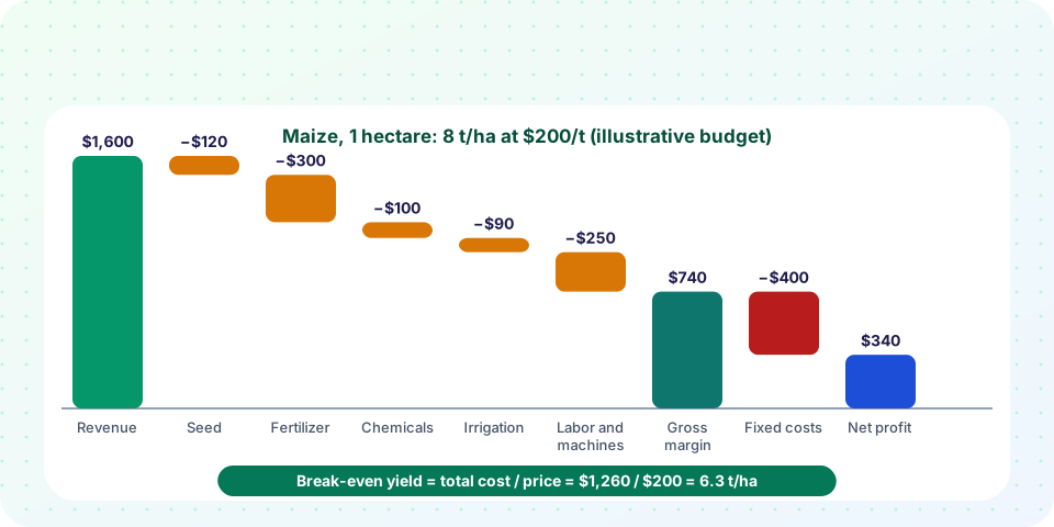
Take one hectare of irrigated maize that yields 8 tonnes and sells at $200 per tonne. The numbers are illustrative:
| Item | $ per hectare |
|---|---|
| Revenue: 8 t × $200 | 1,600 |
| Seed | −120 |
| Fertilizer | −300 |
| Chemicals (herbicide, pesticide) | −100 |
| Irrigation energy | −90 |
| Labor and machinery running costs | −250 |
| Gross margin | 740 |
| Fixed costs (land rent, depreciation, overhead) | −400 |
| Net profit | 340 |
Gross margin is the standard tool for comparing enterprises, because it ignores costs that do not change when you switch crops. If another crop has a gross margin of $900/ha with the same fixed costs, it is the better choice in this simple comparison, provided the risk and the rotation make sense.
Break-even analysis
The break-even yield is the yield at which revenue just covers costs:
break-even yield = total cost / price
With total costs of 860 + 400 = $1,260/ha, the full-cost break-even is 1,260 / 200 = 6.3 t/ha. The yield needed to cover only the variable costs is 860 / 200 = 4.3 t/ha. Below that, planting loses money on every hectare in the short run. Similarly the break-even price at 8 t/ha is 1,260 / 8 = $157.50/t. Knowing these numbers tells a farmer how much room there is for a bad year.
Marginal thinking and partial budgets
Most decisions are about changes, not totals. A partial budget lists only what changes: added returns plus reduced costs, minus added costs and lost returns. The same logic gave the economic optimum for nitrogen: apply an input as long as the extra return is greater than its extra cost.
Investments: discounting and NPV
Money today is worth more than money later, because it can be invested or used now, and because the future is uncertain. A cash flow of C received t years from now is worth C / (1 + r)^t today at a discount rate r. The net present value of a project is the sum of discounted benefits minus the initial cost.
Suppose a drip system costs $2,500 per hectare, lasts 10 years and increases yearly net returns by $450 per hectare (higher yield plus water and labor savings, minus running costs). At a discount rate of 8%:
NPV = −2,500 + 450 × [1 − (1.08)^−10] / 0.08 = −2,500 + 450 × 6.71 ≈ +$520 per hectare
A positive NPV means the investment beats the 8% alternative. The simple payback period is 2,500 / 450 ≈ 5.6 years. Both numbers depend on the assumed benefits, so test them with pessimistic values too. Access to credit, secure land tenure (farmers invest less in land they might lose) and reliable markets often decide whether such investments happen.
Markets: why farm prices swing
For most staple foods, demand is inelastic: people buy about the same amount of rice or wheat whether it is slightly cheaper or dearer. A typical elasticity of staples might be around −0.3 to −0.5. Supply, however, swings with the weather. The result is that small changes in quantity cause big changes in price:
% change in price ≈ % change in quantity / elasticity
If a good harvest raises supply by 10% and elasticity is −0.4, the price falls by about 10 / 0.4 = 25%. Farmers' total revenue then changes by about 1.10 × 0.75 − 1 = −17.5%. A bumper crop can therefore make farmers poorer, a "farmer's paradox". Conversely, a drought can raise prices more than it cuts volume. This is why price volatility is a permanent feature of agriculture, and why governments have often supported farm prices or kept grain reserves.
The cobweb cycle
Because planting decisions are made months before harvest, farmers often base their plans on last year's price. A high price leads to a large planting, a large harvest and a low price, which leads to small planting and a high price again. This is the cobweb model, described by Mordecai Ezekiel in 1938 and often cited for pig and cattle cycles. Whether the cycle fades or grows depends on how strongly supply responds to price compared with how strongly demand does. If supply reacts less than demand, prices settle; if it reacts more, the swings grow.
Managing risk
Farm income is risky: prices, yields, costs, weather, disease and policy all vary. Tools include:
- Diversification: several crops or animals, off-farm income.
- Forward contracts and futures: agreeing a price in advance with a buyer or hedging on a futures market.
- Crop insurance: multi-peril insurance pays for yield losses. Index insurance pays out when a rainfall or satellite index passes a threshold, which avoids field inspections and works for smallholders.
- Storage and timing: selling after the harvest glut, if the farmer can afford to wait.
- Cooperatives: farmers pool produce, share machinery and bargain with buyers; the Amul dairy cooperative in India, begun in Anand in the 1940s, became a model.
- Savings and credit: reliable microfinance prevents distress sales.
Farmers also earn only part of the consumer's price. Processing, transport, marketing and retail take the rest. Shorter chains, certification, contracts and digital market information can raise the farmer's share, but not automatically.
Common misconceptions
"Higher yield always means higher profit." Extra yield is worth it only if the extra revenue is larger than the extra cost, and a bumper crop may lower the price.
"Fixed costs can be ignored." In a single season they do not change the choice between crops, but they decide whether the farm is viable in the long run.
"A positive NPV guarantees success." It depends on the assumptions. Run the numbers with worse yields, prices and discount rates.
Try it
The first program builds the budget above, shows a sensitivity heatmap of net profit across yields and prices, and calculates the drip-system NPV and payback. All figures are illustrative.
Press Run (or Ctrl + Enter) to see the result here.
Program input · what you'd type while the program runs
Type the answers before you press Run, one per line. Each time the program reads a line (with input()), it gets the next line from this box.
The second program simulates the cobweb cycle for three supply responses. Demand is Qd = 100 − 0.5 P; supply planted this year is Qs = 20 + b × P(last year). It is a textbook toy model, not a forecast.
Press Run (or Ctrl + Enter) to see the result here.
Program input · what you'd type while the program runs
Type the answers before you press Run, one per line. Each time the program reads a line (with input()), it gets the next line from this box.
The third tool is a break-even calculator. Enter your own numbers.
Check your understanding
Quick check · 5 questions
of 5 answered You scored / 5 · perfect!
-
1. Revenue is $2,000/ha and variable costs are $1,100/ha. What is the gross margin?
Gross margin = revenue - variable costs = 2,000 - 1,100 = $900/ha. -
2. Total costs are $1,500/ha and the price is $250/t. What is the break-even yield?
1,500 / 250 = 6 t/ha. -
3. Demand elasticity is -0.5 and supply rises 10%. About how far does the price fall?
% change in price = 10 / 0.5 = 20%. -
4. An investment costs $1,000 and gives $300 per year for 5 years at 10%. Is the NPV positive? (Annuity factor 3.79.)
NPV = -1,000 + 300 × 3.79 = -1,000 + 1,137 = +$137. -
5. In the cobweb model, farmers plant based on:
Planting decisions precede harvest, so last year's price drives this year's supply, creating cycles.
Summary
- Gross margin = revenue − variable costs; net profit subtracts fixed costs; break-even yield = total cost / price.
- Decisions are marginal: add an input or change an enterprise only if the extra return exceeds the extra cost.
- NPV discounts future cash flows; a positive NPV beats the discount-rate alternative.
- Inelastic demand makes prices swing with supply; bumper crops can cut revenue, and cobweb cycles arise from lagged planting.
- Diversification, contracts, insurance, cooperatives and credit manage risk.
Track your progress
Create a free account to tick off lessons and pick up where you left off on any device.
of Agricultural Science lessons completed