


















Lesson 36 of 44 · Manifolds and Beyond
Smooth manifolds and tangent spaces
Learn the definition of a smooth manifold through charts and transition maps, see tangent vectors as velocities of curves, and check how components transform with code.
How do you define a surface without saying where it sits? You say how to walk on it. Near every point you want a flat map, a chart, that gives each nearby point a pair of numbers, and you want any two maps that overlap to agree smoothly on how to convert between them. A space with such a system of maps is a smooth manifold. Nothing else is needed: no ambient space, no normal vector.
Once you have charts you can do calculus, and the central tool of calculus on a manifold is the tangent space: at each point, the set of all possible velocities. This lesson builds both ideas from scratch and links them to the surfaces you already know.
What you will learn
- The definition of a smooth manifold: charts, atlas, smooth transition maps.
- The standard examples: circle, sphere, torus and level sets.
- Tangent vectors as velocities of curves and how their components change with the chart.
- The differential of a smooth map and its matrix, the Jacobian.
Key terms
Chart (U, φ): an open set U ⊂ M and a homeomorphism φ: U → φ(U) ⊂ ℝⁿ giving coordinates x¹, …, xⁿ.
Atlas: a collection of charts whose domains cover M.
Transition map: φ_β ∘ φ_α⁻¹, the coordinate change on the overlap of two charts; in a smooth atlas all are infinitely differentiable.
Tangent vector at p: the velocity γ′(0) of a curve with γ(0) = p; the set of them is the tangent space T_p M.
Differential df_p: the linear map T_p M → T_{f(p)} N induced by a smooth map f: M → N.
Charts, atlases and transition maps
A topological manifold of dimension n is a space that is locally like ℝⁿ (every point lies in a chart), Hausdorff (distinct points can be separated) and not too large (second countable). A smooth manifold adds a smooth atlas: for any two charts (U, φ) and (V, ψ) with U ∩ V ≠ ∅, the transition map
ψ ∘ φ⁻¹ : φ(U ∩ V) → ψ(U ∩ V)
is smooth (all derivatives exist) with a smooth inverse. This is how calculus survives change of coordinates: a function is smooth if it is smooth in every chart, and the compatibility guarantees the answer is the same in all of them.
Examples
ℝⁿwith the identity chart.- The circle
S¹: no single chart (a chart on the whole circle would be a homeomorphism to an interval), but two angle charts, or two stereographic charts, do it. - The sphere
S²: stereographic projections from the north and south poles. Forp = (x, y, z),φ_N(p) = (x, y)/(1 − z)andφ_S(p) = (x, y)/(1 + z). Forw = φ_N(p)one findsφ_S(p) = w/|w|², so the transition map is inversion in the unit circle: smooth onℝ² ∖ {0}. - Products. The torus
T² = S¹ × S¹has charts that are products of charts of the circle. - Level sets. If
F: ℝ³ → ℝis smooth and∇F ≠ 0on the setF = c, that set is a smooth surface. The sphere isx² + y² + z² = 1. - Graphs of smooth functions
z = f(x, y), the surfaces of the first chapters.
A map between manifolds is smooth if it is smooth when written in charts. A smooth map with smooth inverse is a diffeomorphism: two manifolds related by one are the same smooth manifold. (For example, an egg and a sphere are diffeomorphic.)
Tangent vectors
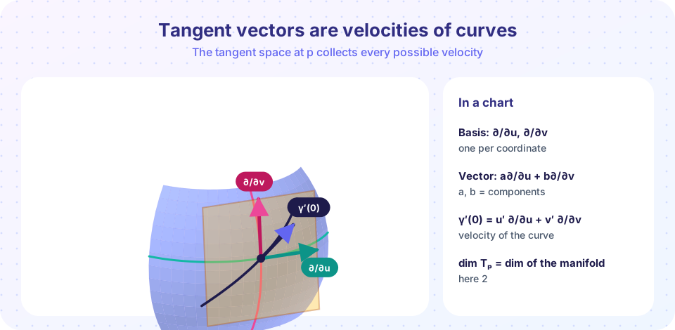
Let γ: (−ε, ε) → M be a smooth curve with γ(0) = p. In a chart x = (x¹, …, xⁿ) it has coordinate functions xⁱ(γ(t)), and its velocity components are
vⁱ = d/dt xⁱ(γ(t)) at t = 0.
Two curves with the same components in one chart have the same components in every chart (by the chain rule), so we treat them as the same tangent vector. The set of all such velocities is the tangent space T_p M, an n-dimensional vector space with the coordinate basis
∂/∂x¹, …, ∂/∂xⁿ (velocities of the coordinate lines through p),
so that v = Σ vⁱ ∂/∂xⁱ. For a surface x(u, v) in ℝ³, ∂/∂u corresponds to xᵤ and ∂/∂v to xᵥ: the tangent plane of the first chapters is this tangent space.
Changing coordinates
If y = y(x) is another chart, the same vector has components
wʲ = Σᵢ (∂yʲ/∂xⁱ) vⁱ,
that is, the Jacobian of the transition map acts on components. This is the rule that defines what a vector is: something whose components change by the Jacobian. It explains why the velocity of a curve is a well-defined geometric object, even though its numbers depend on the chart.
Vectors as derivatives
A vector v also acts on smooth functions: v(f) = d/dt f(γ(t)) at t = 0 = Σ vⁱ ∂f/∂xⁱ. This directional derivative is how tangent vectors are often defined in modern texts: as operators satisfying the product rule.
The differential of a map
For a smooth map f: M → N, a curve γ in M goes to the curve f ∘ γ in N. The velocity of the new curve defines
df_p(v) = (f ∘ γ)′(0).
In charts, df_p has matrix the Jacobian ∂fʲ/∂xⁱ. The chain rule d(g ∘ f) = dg ∘ df follows. If df_p is invertible, f is a local diffeomorphism near p. The transition-map rule above is the special case where f is the identity of M written in two charts.
Vector fields. A smooth assignment p ↦ X(p) ∈ T_p M is a vector field. Its integral curves (paths that follow the arrows) solve ordinary differential equations: the geodesic equation of the last chapter is one, written for a field on the tangent bundle.
Common misconceptions
"Tangent vectors live in the surrounding space." For surfaces in ℝ³ we can draw them that way, but intrinsically a tangent vector is a velocity, and T_p M exists even when there is no surrounding space.
"Vectors at different points can be added." Only vectors in the same tangent space can be. Comparing T_p M and T_q M needs extra structure, such as parallel transport.
"The components of a vector are intrinsic." The numbers vⁱ depend on the chart; what is intrinsic is the vector itself, and the rule wʲ = (∂yʲ/∂xⁱ) vⁱ.
Try it
First, check the transformation rule numerically. Take a curve on the unit sphere, compute its velocity in the northern and southern stereographic charts by finite differences, and verify that the Jacobian of the transition w ↦ w/|w|² carries one into the other.
Press Run (or Ctrl + Enter) to see the result here.
Program input · what you'd type while the program runs
Type the answers before you press Run, one per line. Each time the program reads a line (with input()), it gets the next line from this box.
The two sets of numbers differ, but J · vN = vS: the vector is the same, only its components changed. Second, draw how a chart sees the sphere: parallels become circles and meridians become rays in the stereographic plane of chart N.
Press Run (or Ctrl + Enter) to see the result here.
Program input · what you'd type while the program runs
Type the answers before you press Run, one per line. Each time the program reads a line (with input()), it gets the next line from this box.
Note the label: with polar angle θ measured from the north pole, the equator θ = 90° has ρ = 1, and θ → 0 (near the north pole, the projection point) goes to infinity. Last, a live picture of the two charts of the circle.
The dashed lines project the point from the north pole (teal) and the south pole (pink) onto the horizontal line; the product of the two coordinates is always 1, which is the one-dimensional transition map w ↦ 1/w. (Near the ends of the line the dot is clipped to the drawing area.)
Check your understanding
Quick check · 5 questions
of 5 answered You scored / 5 · perfect!
-
1. The transition map between two charts of a smooth manifold must be
That compatibility is what makes calculus independent of the chart. -
2. A tangent vector at p can be defined as
T_p M is the set of velocities of curves through p. -
3. If y = y(x) is a change of coordinates, the components of a tangent vector change by
wʲ = Σ (∂yʲ/∂xⁱ) vⁱ. -
4. The dimension of the tangent space of the torus at any point is
dim T_p M = dim M = 2 for a surface. -
5. The differential df_p of a smooth map f in charts is represented by
df_p is the linear map whose matrix is the matrix of first partial derivatives.
Summary
- A smooth manifold is covered by charts whose transition maps are smooth; no ambient space is needed.
- Examples:
ℝⁿ, the circle and sphere (two charts), products such as the torus, level sets and graphs. - Tangent vectors are velocities of curves;
T_p Mhas the coordinate basis∂/∂xⁱand components change by the Jacobian. - The differential
df_pis the Jacobian in charts; the chain rule holds.
Track your progress
Create a free account to tick off lessons and pick up where you left off on any device.
of Differential Geometry lessons completed