


















Lesson 37 of 44 · Manifolds and Beyond
Riemannian metrics and the curvature tensor
Put a metric on a manifold, recover lengths, geodesics and parallel transport in any dimension, and compute Riemann, Ricci and scalar curvature for spheres and the hyperbolic plane.
A manifold by itself has no lengths, angles or curvature: it only knows which functions are smooth. To measure, you must add an inner product on every tangent space, varying smoothly from point to point. That choice is a Riemannian metric, and it is the generalization of the first fundamental form. Once you have it, everything from the chapters on surfaces comes back: lengths of curves, geodesics, parallel transport, and, with one new idea, curvature in every dimension.
The new idea is that curvature in dimension 3 and up cannot be one number or even two. At a point of a 3-dimensional manifold there is a whole family of directions of 2-dimensional "slices", each with its own bending. The Riemann curvature tensor packages all of them.
What you will learn
- What a Riemannian metric is and how it gives lengths, angles and volumes.
- How Christoffel symbols, geodesics and parallel transport carry over from surfaces.
- How to compute the Riemann, Ricci and scalar curvatures, with code.
- What the curvature of the sphere and of the hyperbolic plane look like in this language.
Key terms
Riemannian metric g: a smooth choice of inner product g_p on each tangent space; in coordinates a symmetric positive-definite matrix gᵢⱼ(x).
Levi-Civita connection: the unique torsion-free connection compatible with g, whose Christoffel symbols are given by the same formula as on surfaces.
Riemann tensor Rρσμν: measures the failure of parallel transport around infinitesimal loops.
Ricci tensor and scalar curvature: traces of the Riemann tensor, R_{σν} = Rρσρν and R = gσν R_{σν}.
Sectional curvature K(u, v): the Gaussian curvature of the surface swept by geodesics tangent to the plane spanned by u, v.
The metric
A Riemannian metric in coordinates is ds² = gᵢⱼ dxⁱ dxʲ. For a surface it is E du² + 2F du dv + G dv². With it:
- the length of a curve is
∫ √(gᵢⱼ ẋⁱ ẋʲ) dt; - the angle between vectors is
cos θ = g(u, v)/(|u||v|); - the volume element is
√(det g) dx¹ ⋯ dxⁿ.
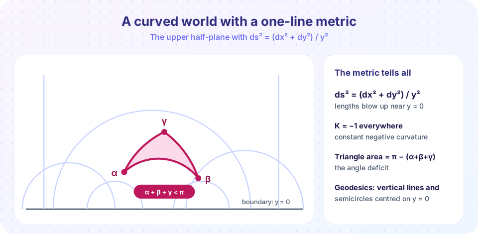
Examples: Euclidean space δᵢⱼ; the unit sphere dθ² + sin²θ dφ²; the hyperbolic half-plane ds² = (dx² + dy²)/y² on y > 0; the 3-sphere of radius 1 dχ² + sin²χ (dθ² + sin²θ dφ²). Every manifold admits a Riemannian metric (by gluing local ones with a partition of unity), so the existence is never in doubt; the interesting question is which metrics are special.
Connection, geodesics and transport
Define
Γᵏᵢⱼ = ½ gᵏˡ ( ∂ᵢ g_{jl} + ∂ⱼ g_{il} − ∂ₗ g_{ij} ).
Exactly as on a surface, geodesics solve ẍᵏ + Γᵏᵢⱼ ẋⁱ ẋʲ = 0 and a vector field W is parallel along a curve when Ẇᵏ + Γᵏᵢⱼ ẋⁱ Wʲ = 0. Nothing changes except that i, j, k now run over 1, …, n. Both are intrinsic: they depend on g alone.
The Riemann curvature tensor
On a surface, curvature was the rotation after going around a small loop. In general we measure how parallel transport around the infinitesimal parallelogram spanned by ∂ᵤ and ∂ᵥ fails to be the identity. The result, in coordinates (with the convention in which spheres have positive curvature), is
Rρσμν = ∂μ Γρνσ − ∂ν Γρμσ + Γρμλ Γλνσ − Γρνλ Γλμσ.
Contracting once gives the Ricci tensor R_{σν} = Rρσρν; contracting again with the inverse metric gives the scalar curvature R = gσν R_{σν}.
Surfaces recovered
For a 2-dimensional manifold all curvature information is one function: R_{σν} = K g_{σν} and R = 2K, where K is the Gaussian curvature. So the unit sphere has Ricci = g and R = 2; a sphere of radius a has K = 1/a² and R = 2/a².
Sectional curvature and space forms
For two independent tangent vectors u, v, the sectional curvature is K(u, v) = g(R(u, v)v, u) / (|u|²|v|² − g(u, v)²), the Gaussian curvature of the surface swept by geodesics leaving p in the directions of the plane. A manifold of constant sectional curvature κ is a space form:
| Space | Sectional curvature | Ricci | Scalar curvature |
|---|---|---|---|
Euclidean ℝⁿ |
0 |
0 |
0 |
Sphere Sⁿ of radius a |
1/a² |
(n − 1)/a² · g |
n(n − 1)/a² |
Hyperbolic space Hⁿ |
−1 |
−(n − 1) g |
−n(n − 1) |
Worked example: the hyperbolic half-plane
The metric ds² = (dx² + dy²)/y² is conformal to the flat one: g = e^{2φ}(dx² + dy²) with φ = −ln y. For a conformally flat surface the Gaussian curvature is K = −e^{−2φ} Δφ with Δ the ordinary Laplacian. Here Δφ = ∂²φ/∂y² = 1/y² and e^{−2φ} = y², so K = −1 everywhere. The nonzero Christoffel symbols are Γˣₓᵧ = −1/y, Γʸₓₓ = 1/y, Γʸᵧᵧ = −1/y, and the geodesic equations are
x″ = 2x′y′/y, y″ = (y′² − x′²)/y.
Their solutions are vertical lines and semicircles centered on the x-axis, the pictured geodesics. The distance between (x₁, y₁) and (x₂, y₂) is arccosh(1 + ((x₂ − x₁)² + (y₂ − y₁)²)/(2 y₁ y₂)).
Why this matters. General relativity models spacetime as a 4-dimensional manifold whose metric has one negative direction (Lorentzian signature). Freely falling particles follow geodesics, and Einstein's equation sets a combination of the Ricci tensor and scalar curvature equal to the energy content. See the Relativity track for the physics.
Common misconceptions
"Curvature is one number at each point." Only in dimension 2. In dimension n the Riemann tensor has n²(n² − 1)/12 independent components; the Ricci tensor and scalar curvature are partial summaries.
"The Riemann tensor is built from the Christoffel symbols, and those are tensors." Christoffel symbols are not tensors, but the combination in the Riemann tensor is: its components transform correctly under change of coordinates.
"Zero Ricci curvature means flat." Not in dimension 3 and up. Ricci-flat manifolds can still have nonzero Riemann curvature (in dimension 4 this is where gravitational waves and black holes live). In dimension 2 and 3 Ricci-flat does imply flat.
Try it
First compute the Christoffel symbols and the Riemann, Ricci and scalar curvatures symbolically for any metric, and test them on the spaces in the table.
Press Run (or Ctrl + Enter) to see the result here.
Program input · what you'd type while the program runs
Type the answers before you press Run, one per line. Each time the program reads a line (with input()), it gets the next line from this box.
The scalar curvatures are 2, 1/2, −2, 0 and 6, matching the table (n(n − 1)/a² for spheres, −n(n − 1) for hyperbolic space), and in each case the Ricci tensor is a multiple of the metric. Second, solve the geodesic equations of the half-plane and check that the paths are semicircles centered on the axis.
Press Run (or Ctrl + Enter) to see the result here.
Program input · what you'd type while the program runs
Type the answers before you press Run, one per line. Each time the program reads a line (with input()), it gets the next line from this box.
Every path lies on a circle centered on the x-axis (deviation near zero), except the vertical one. Third, a distance calculator for the half-plane: drag two points and see the geodesic and its hyperbolic length.
The pink arc is the geodesic; the grey dashed straight segment is longer in the hyperbolic metric because it stays near the boundary where 1/y is large.
Check your understanding
Quick check · 6 questions
of 6 answered You scored / 6 · perfect!
-
1. A Riemannian metric on a manifold is
gₚ(u, v) defines lengths and angles at each point and varies smoothly. -
2. The Christoffel symbols in any dimension are given by
This is the same formula as for surfaces, with indices running over 1, …, n. -
3. For a surface, the scalar curvature R is
Ricci = K g, and the trace of g with itself is 2. -
4. The hyperbolic half-plane (dx² + dy²)/y² has Gaussian curvature
K = −e^{−2φ}Δφ = −y²·(1/y²) = −1. -
5. The scalar curvature of the unit n-sphere is
Sectional curvature 1 in every plane: n(n − 1) planes' worth, giving R = n(n − 1). -
6. Geodesics of the half-plane are
Those are the solutions of the geodesic equations, as the numerical experiment shows.
Summary
- A Riemannian metric
ggives lengths, angles and volumes on a manifold; Christoffel symbols, geodesics and parallel transport are defined exactly as for surfaces. - The Riemann tensor measures failure of parallel transport around small loops; Ricci and scalar curvature are traces. In dimension 2,
Ricci = K gandR = 2K. - Space forms:
ℝⁿ(0),Sⁿ(1/a²),Hⁿ(−1), with scalar curvatures0,n(n − 1)/a²,−n(n − 1). - The half-plane metric
(dx² + dy²)/y²hasK = −1, geodesics that are semicircles, and triangles with angle sum less thanπ.
Next: Chapter 8 review
Track your progress
Create a free account to tick off lessons and pick up where you left off on any device.
of Differential Geometry lessons completed