


















Lesson 29 of 44 · Geodesics
Parallel transport and holonomy
Carry a vector along a curve without turning it, see why it returns rotated after a loop on a sphere, and verify that the rotation equals the enclosed Gaussian curvature.
On a flat sheet of paper, you can carry an arrow from one place to another without any ambiguity: just keep it pointing the same way. The result does not depend on the route you take. On a curved surface that changes. Carry an arrow along two different routes between the same two points and the two copies may point in different directions.
That strange fact is the cleanest way to see curvature. You do not need formulas to feel it: walk around a loop on a sphere, holding an arrow as steadily as you can, and when you get back it has turned. The amount it turned is exactly the total Gaussian curvature inside the loop. This lesson makes the idea precise and checks it numerically.
What you will learn
- What it means for a vector field along a curve to be parallel.
- The coordinate equations of parallel transport.
- What holonomy is and how it relates to
Kand area. - How to compute holonomy numerically on a sphere and check it against theory.
Key terms
Covariant derivative DW/dt: the derivative of a tangent vector field W along a curve, with the normal component thrown away (the tangential part of dW/dt).
Parallel vector field: a tangent field W along α with DW/dt = 0.
Parallel transport: carrying a vector along a curve by solving DW/dt = 0 with a given starting vector.
Holonomy: the rotation between the starting vector and the vector that returns after transporting around a closed loop.
Levi-Civita connection: the name for this rule of differentiating tangent fields; it is built from the metric alone.
The idea
Take a curve α(t) on a surface and a tangent vector field W(t) along it. Differentiate W as a vector in space: dW/dt. This derivative has a tangential part and a normal part. The normal part is only the surface bending away beneath your feet; the tangential part is the change that someone living on the surface would notice. Define
DW/dt = (dW/dt)_tangential
and call W parallel if DW/dt = 0. Three facts follow.
- Length and angle are preserved. For two parallel fields,
d/dt ⟨W₁, W₂⟩ = ⟨DW₁/dt, W₂⟩ + ⟨W₁, DW₂/dt⟩ = 0, so lengths and angles between them are constant. - Geodesics are the curves whose tangent is parallel.
DT/dt = 0means exactly thatα″has no tangential part. - Transport is intrinsic. In coordinates
W = W¹ xᵤ + W² xᵥ,
dWᵏ/dt + Σ Γᵏᵢⱼ (duⁱ/dt) Wʲ = 0.
This is a linear ODE, so a starting vector gives exactly one parallel field. Only the Christoffel symbols, hence only E, F, G, appear.
Transport is linear and isometric: the map P: T_{α(0)}S → T_{α(1)}S that carries a starting vector to its transported copy is a rotation (possibly composed with a reflection, never with orientation reversal on an oriented surface).
Holonomy
Transport a vector around a closed loop. It comes back as P(W), a rotation of W by some angle Δ. This angle is the holonomy of the loop. In the plane Δ = 0 for every loop. On a surface with K ≠ 0, for a simple loop bounding a region R,
Δ ≡ ∬_R K dA (mod 2π)
with the sign positive for a counterclockwise loop. This is a first, quantitative sense in which curvature is accumulated rotation.
Worked example 1: the octant
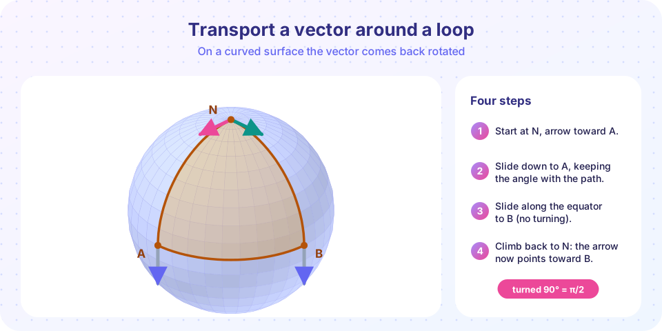
On the unit sphere take the triangle with vertices N (north pole), A on the equator at longitude 0 and B on the equator at longitude 90°. All sides are geodesics and all three angles are 90°. Its area is 4π/8 = π/2, and K = 1, so Δ = π/2. Follow the arrow from the picture:
- At
Nthe arrow points towardA. Slide down the meridian toA: the arrow stays tangent to the path, pointing south. - Move along the equator from
AtoB. The arrow stays perpendicular to the equator, still pointing south. - Climb the meridian of
BtoN. Now the arrow is the reverse of the direction of travel, so atNit points towardB.
The arrow started toward A (longitude 0) and ended toward B (longitude 90°): a quarter turn, π/2, as predicted.
Worked example 2: a circle of latitude
Let the loop be the circle at polar angle θ₀ on the unit sphere, traversed once. It bounds the cap of area 2π(1 − cos θ₀), so Δ = 2π(1 − cos θ₀) (mod 2π). For θ₀ = 90° (the equator, a geodesic) Δ = 2π ≡ 0: transport along a geodesic keeps the same angle to the path and the arrow returns unchanged. For θ₀ = 45°, Δ = 2π(1 − 0.7071) ≈ 1.840 radians, about 105°.
The transport equations along this circle (u = θ₀, v = t) reduce to W¹′ = sin θ₀ cos θ₀ · W² and W²′ = −cot θ₀ · W¹. In an orthonormal frame the arrow turns at constant rate cos θ₀ per radian of longitude, so over a full lap it turns by 2π cos θ₀, and 2π cos θ₀ ≡ −2π(1 − cos θ₀) (mod 2π): the same magnitude, with the sign telling you the direction relative to the frame.
Foucault's pendulum. A pendulum's swing plane is carried along the latitude circle by (almost) parallel transport. Its plane turns, relative to the ground, by about 360° · sin(latitude) per day. This is the holonomy formula above written for θ₀ = 90° − latitude.
Common misconceptions
"Parallel transport keeps the vector pointing in a fixed direction in space." The vector in space changes: it must stay tangent to the surface as the tangent plane tilts. What stays fixed is the angle with the path (along geodesics), as measured by someone on the surface.
"Holonomy only depends on where the loop starts." It depends only on the loop and on its orientation, not on the starting point (up to expressing the angle in a different tangent plane).
"Holonomy is zero when K = 0." For loops that bound a flat patch, yes. On a round cylinder it is zero even for a loop that goes around the tube, because transport there is the same as on the unrolled strip. A cone is different: a loop around the apex, where the surface is not smooth, is rotated by the angle defect of the apex.
Try it
First, solve the transport equations numerically along circles of latitude and compare with 2π(1 − cos θ₀).
Press Run (or Ctrl + Enter) to see the result here.
Program input · what you'd type while the program runs
Type the answers before you press Run, one per line. Each time the program reads a line (with input()), it gets the next line from this box.
The dots lie on the curve: the transport equations, which use only the metric, reproduce ∬K dA. Second, test the octant and arbitrary spherical triangles with a completely different method: discrete transport by projection. At each small step we project the vector onto the new tangent plane and renormalize.
Press Run (or Ctrl + Enter) to see the result here.
Program input · what you'd type while the program runs
Type the answers before you press Run, one per line. Each time the program reads a line (with input()), it gets the next line from this box.
The loop's holonomy equals the enclosed spherical area (K = 1), with the sign of the orientation. Last, an interactive dial.
This dial is a visual of the formula Δ = ∬K dA for the unit sphere, not a simulation of transport.
Check your understanding
Quick check · 5 questions
of 5 answered You scored / 5 · perfect!
-
1. A vector field W along a curve is parallel if
DW/dt is the tangential part of dW/dt; parallel means DW/dt = 0. -
2. Transport a vector around the octant triangle on the unit sphere. It returns rotated by
The enclosed area is π/2 and K = 1, so the holonomy is π/2. -
3. Along a geodesic, the tangent vector is
DT/dt = 0 is the definition of a geodesic in terms of parallel transport. -
4. Parallel transport preserves
⟨W₁, W₂⟩ is constant along the curve, so lengths and angles do not change. -
5. For a simple loop on a surface, the holonomy angle (mod 2π) equals
This is the first form of the relation between holonomy and Gaussian curvature.
Summary
- Parallel transport keeps
DW/dt = 0(tangential derivative zero); it preserves lengths and angles and is built from the Christoffel symbols. - Geodesics are the curves whose tangent vector is parallel along them.
- Holonomy is the rotation after a loop; for a simple loop it equals
∬K dA(mod 2π). - Octant of the sphere:
π/2; latitude circle at polar angleθ₀:2π(1 − cos θ₀). - The plane has zero holonomy: transport there is path-independent.
Next: Chapter 6 review
Track your progress
Create a free account to tick off lessons and pick up where you left off on any device.
of Differential Geometry lessons completed