


















Lesson 39 of 44 · Projects and Practice
Project: curvature of a triangle mesh
Build a sphere mesh and a torus mesh, estimate Gaussian curvature from angle defects and mean curvature from the cotangent Laplacian, and compare with exact formulas.
Real shapes in graphics, medicine and engineering come as triangle meshes: lists of vertices and triangles, with no formula behind them. Yet the questions of this course, how curved is it here, still make sense. In this project you will turn two ideas from the previous chapters into working code: the angle defect from the Gauss–Bonnet chapter gives Gaussian curvature, and the cotangent Laplacian gives mean curvature. You will test both on surfaces whose exact curvature you know, so you can see how accurate they are.
What you will learn
- How to compute per-vertex angle defects and area shares with vectorized NumPy.
- How the cotangent weights give the mean curvature vector.
- How to validate a numerical method against exact results, and what errors look like.
- How mesh quality (regular or irregular vertices) changes the answer.
Key terms
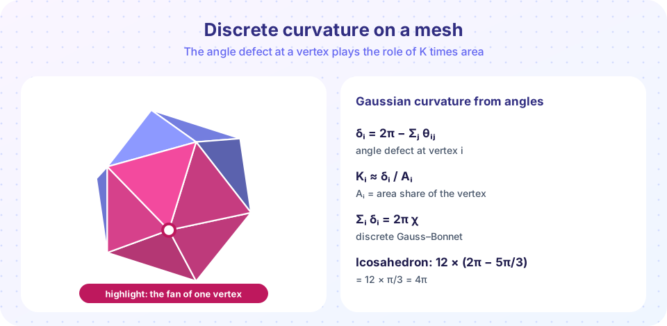
Angle defect δᵢ: 2π minus the sum of the triangle angles at vertex i.
Vertex area Aᵢ: one third of the total area of the triangles around vertex i (the "barycentric" share).
Discrete Gaussian curvature: Kᵢ ≈ δᵢ / Aᵢ.
Cotangent weights: for the edge between vertices i and j, cot αᵢⱼ + cot βᵢⱼ, where α, β are the angles opposite the edge in the two triangles that share it.
Mean curvature vector: ½ Δ x where Δ xᵢ = (1/(2Aᵢ)) Σⱼ (cot αᵢⱼ + cot βᵢⱼ)(xⱼ − xᵢ) approximates −2H n.
The plan
- Build a mesh: an icosphere (an icosahedron whose triangles are repeatedly split and pushed onto a sphere) and a torus grid.
- For each triangle compute its three angles and its area.
- Add up the angles and the area shares at each vertex, giving
δᵢandAᵢ. - Accumulate cotangent-weighted edge vectors for the mean curvature vector.
- Compare with
K = 1/R²,|H| = 1/Ron the sphere and with the torus formulasK = cos v / (r(R + r cos v)),|H| = |R + 2r cos v| / (2r(R + r cos v)). - Check the discrete Gauss–Bonnet theorem:
Σ δᵢ = 2πχ.
Why does the angle defect work? On a smooth surface a small disk of area A around a point is "short" in circumference compared with a flat disk by an amount proportional to K, and the sum of the angles around a vertex of a polyhedral surface falls short of 2π by the defect: it is the integral of K over the vertex's cell. So δᵢ ≈ ∬K dA ≈ Kᵢ Aᵢ.
Why does the cotangent Laplacian work? For a smooth surface the Laplace–Beltrami operator applied to the position function x gives Δ x = −2 H n (with the sign convention that makes H positive for the outward normal of a sphere, up to orientation). The cotangent formula is the standard finite-element discretization of that operator. On a sphere of radius R, |Δ x| = 2/R, hence |H| = 1/R.
Try it
Everything needs vectors, so we use NumPy. The code below builds both meshes, computes the per-vertex values and prints how far they are from the truth.
Press Run (or Ctrl + Enter) to see the result here.
Program input · what you'd type while the program runs
Type the answers before you press Run, one per line. Each time the program reads a line (with input()), it gets the next line from this box.
Read the output. The sphere's mean values are within a fraction of a percent of 1/R² = 0.25 and 1/R = 0.5. The maximum K is larger because the 12 original vertices of the icosahedron have 5 neighbors instead of 6: mesh irregularity produces the biggest errors. The sum of defects is 4π to eight digits and 0 on the torus: that is the discrete Gauss-Bonnet theorem, exact for any mesh, however rough.
Now study convergence. We refine the sphere mesh and track the error, then plot the torus estimates against the exact curve.
Press Run (or Ctrl + Enter) to see the result here.
Program input · what you'd type while the program runs
Type the answers before you press Run, one per line. Each time the program reads a line (with input()), it gets the next line from this box.
The estimates sit on the exact curve for the torus (the grid is regular), and on the sphere the RMS error halves each time the number of vertices quadruples (that is, each time the edge length halves), from about 0.31 at the bare icosahedron to about 0.01 after four refinements. Last, look at why the defect measures curvature. Surround a vertex with n equilateral triangles (each contributes 60°) and see what happens.
For n = 6 the triangles tile the plane, for n < 6 there is a gap you can close by folding (a cone, like a corner of an icosahedron with n = 5), and for n > 6 the flattened triangles overlap, a surface with too much room, like a saddle. This drawing shows the angle bookkeeping for equilateral triangles only.
Extensions to try
- Add noise to the vertex positions and watch the estimates break down; then smooth them by averaging
Kover the neighbors. - Replace the barycentric area by the Voronoi area for obtuse-triangle robustness.
- Sort the vertices by
Kand use the sign to color the mesh (teal, yellow, pink) as in the torus picture of Chapter 5. - Estimate
κ₁, κ₂ = H ± √(H² − K)per vertex.
Check your understanding
Quick check · 4 questions
of 4 answered You scored / 4 · perfect!
-
1. The angle defect at a vertex is
On a flat mesh the angles sum to 2π and the defect is 0. -
2. The sum of the angle defects over all vertices of a closed triangle mesh is
Discrete Gauss-Bonnet: 4π for spheres, 0 for tori. -
3. On the icosphere the largest curvature errors appear at
Irregular vertices (valence other than 6) break the symmetry of the discretization. -
4. Six equilateral triangles around a vertex give
6 × 60° = 360°, defect 0.
Summary
- Gaussian curvature of a mesh:
Kᵢ ≈ δᵢ / Aᵢwithδᵢ = 2π − Σ anglesandAᵢone third of the surrounding area. - Mean curvature: half the length of the cotangent Laplacian of the position vector.
- The defects obey Gauss–Bonnet exactly:
Σ δᵢ = 2πχ. - Accuracy depends on mesh quality: irregular vertices and noise produce the largest errors.
Track your progress
Create a free account to tick off lessons and pick up where you left off on any device.
of Differential Geometry lessons completed