


















Lesson 4 of 44 · Getting Started
Plotting Curves and Surfaces with Python
Learn the three plotting recipes used in every lesson: sampling a curve, building a surface grid with meshgrid, and drawing tangent vectors with quiver.
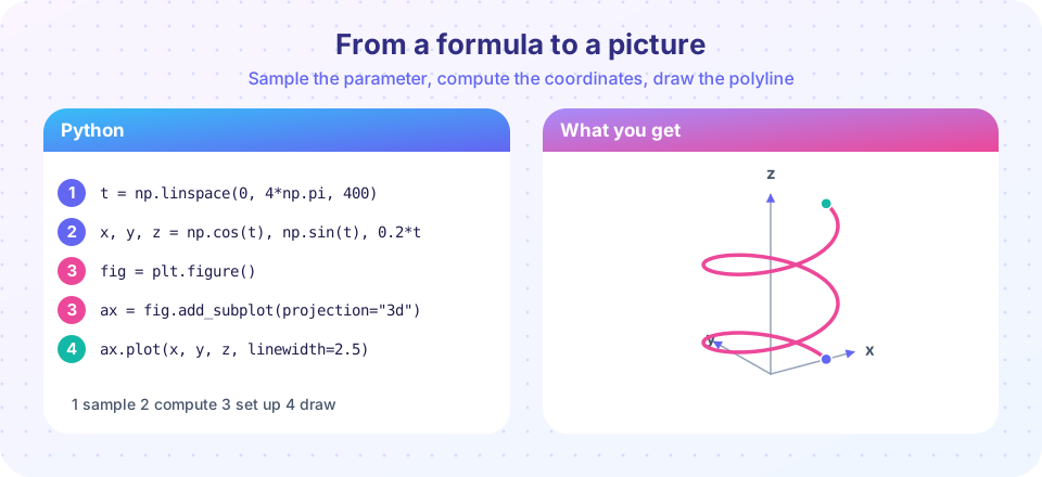
Geometry is a visual subject, and the quickest way to build intuition is to draw things and change them. This lesson shows the three recipes that every later lesson uses: sample a parametrized curve, sample a parametrized surface on a grid, and draw vectors on top. We use numpy for the numbers and matplotlib for the pictures; both run in your browser here.
What you will learn
- How to sample a parametric curve with
np.linspaceand draw it in 2D and 3D - How to build a surface grid with
np.meshgridand draw it withplot_surface - How to draw tangent vectors with
quiver - How to check a plot against a number, such as a polyline length
Key terms
Sampling: choosing a finite list of parameter values, such as 400 equally spaced values of t.
Polyline: the broken line obtained by joining sampled points with straight segments.
Meshgrid: two 2D arrays that hold every combination of u and v values.
Quiver: a plot made of arrows, used here for tangent vectors.
Recipe 1: a parametrized curve
A parametrized curve is a function t → (x(t), y(t), z(t)). In code, t is an array, and the three coordinates are three arrays of the same length. Plotting joins consecutive points with straight segments, so the more samples you take, the smoother the picture.
t = np.linspace(0, 2*np.pi, 400)     # 400 values from 0 to 2π
x, y = np.cos(t), np.sin(t)          # unit circle
plt.plot(x, y)
Rules of thumb: use a few hundred samples for smooth curves; remember np.linspace(a, b, n) includes both endpoints; and call ax.set_aspect("equal") for plane curves so circles look like circles.
In the Try it section below, the first program draws three famous plane curves from their parametrizations: a circle, a cycloid and a three-petal rose. Edit the formulas to explore.
Recipe 2: a parametrized surface
A surface patch is a function (u, v) → (x, y, z). We sample a grid of u and v values with np.meshgrid, compute X, Y, Z arrays of the same shape, and hand them to plot_surface. The grid lines you see on the plot are the coordinate curves u = const and v = const, the same lines that fill the pictures in this course. For a torus with big radius a and tube radius b:
x = (a + b cos v) cos u, y = (a + b cos v) sin u, z = b sin v
Recipe 3: tangent vectors with quiver
Differentiate by hand (or with np.gradient), then draw arrows. In 3D use ax.quiver(x, y, z, dx, dy, dz, length=...). The second program draws a trefoil knot and its unit tangent vectors; the arrows show the direction of travel.
Check a plot with a number
Pictures can hide errors, so we also check numerically. The length of a polyline through sampled points is np.sum(np.linalg.norm(np.diff(points), axis=...)). For the helix (cos t, sin t, t) on 0 ≤ t ≤ 2π the exact length is 2π√2 ≈ 8.8858. The polyline length is slightly smaller (straight chords cut corners) and approaches the exact value as you add samples. This is the numerical shadow of the arc-length integral you will meet in chapter 2.
Press Run (or Ctrl + Enter) to see the result here.
Program input · what you'd type while the program runs
Type the answers before you press Run, one per line. Each time the program reads a line (with input()), it gets the next line from this box.
Common misconceptions
"More samples are always better." More samples give smoother pictures but cost time and memory. A few hundred points suffice for a curve and a 40 by 80 grid for a surface.
"The plot is the curve." A plot is a polyline approximation. If a curve has a sharp cusp or very fast turn and you sample sparsely, the picture can look wrong even though the formula is right.
"Axes are always equal." 3D plots stretch axes by default. Use ax.set_box_aspect((1, 1, 1)) (or the exact ranges) when shape matters.
Try it
Press Run (or Ctrl + Enter) to see the result here.
Program input · what you'd type while the program runs
Type the answers before you press Run, one per line. Each time the program reads a line (with input()), it gets the next line from this box.
Press Run (or Ctrl + Enter) to see the result here.
Program input · what you'd type while the program runs
Type the answers before you press Run, one per line. Each time the program reads a line (with input()), it gets the next line from this box.
Press Run (or Ctrl + Enter) to see the result here.
Program input · what you'd type while the program runs
Type the answers before you press Run, one per line. Each time the program reads a line (with input()), it gets the next line from this box.
Check your understanding
Quick check · 4 questions
of 4 answered You scored / 4 · perfect!
-
1. What does np.linspace(0, 1, 5) return?
linspace includes both endpoints and spaces the five values evenly, so the step is 0.25. -
2. What does np.meshgrid(u, v) produce?
Each output array has one entry per grid point, ready for computing X, Y, Z. -
3. A polyline through points on a smooth curve is usually...
A straight chord is the shortest path between its endpoints, so a polyline cuts corners. -
4. Why call ax.set_aspect('equal') on a plane curve?
Without equal aspect, the x and y scales differ and shapes look stretched.
Summary
- A curve is sampled with
np.linspace; a surface patch withnp.meshgridon(u, v). plotdraws curves,plot_surfacesurfaces,quiverarrows.- Polylines approximate curves; the approximation improves with more samples.
- Check pictures with numbers (like polyline length) whenever you can.
Next: Chapter 1 Review
Track your progress
Create a free account to tick off lessons and pick up where you left off on any device.
of Differential Geometry lessons completed