


















Lesson 40 of 44 · Projects and Practice
Project: build a geodesic solver
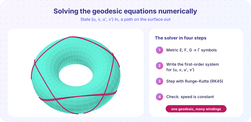
Write a general geodesic solver that takes any parametrized surface, computes Christoffel symbols symbolically, integrates numerically and finds shortest paths by shooting.
In Chapter 6 you solved the geodesic equations by hand for a few surfaces. In this project you will write one program that does it for any surface given by a formula x(u, v). It computes the metric, derives the Christoffel symbols symbolically, integrates the equations numerically, and then solves the practical problem: given two points on a surface, find the geodesic that joins them.
The structure of the program mirrors the theory, which makes it a good review. The metric comes from the first fundamental form, the symbols from the formula for Γᵏᵢⱼ, the path from the geodesic equation and the endpoints from a root-finding step called shooting.
What you will learn
- How to turn the geodesic equations into a reusable solver with sympy and SciPy.
- How to test a solver against conservation laws (constant speed, Clairaut's constant).
- How to solve a boundary-value problem by shooting.
- Why a geodesic joining two points is shorter than the straight line in the parameter plane.
The design
| Step | What it does | Theory behind it |
|---|---|---|
| 1 | Compute E, F, G from x(u, v) with sympy |
first fundamental form |
| 2 | Build Γᵏᵢⱼ = ½ gᵏˡ(∂ᵢg_{jl} + ∂ⱼg_{il} − ∂ₗg_{ij}) |
Levi-Civita connection |
| 3 | Write the state (u, v, u′, v′) and u″ = −Γ u′u′ |
geodesic equations |
| 4 | Start with unit speed in the metric | geodesics have constant speed |
| 5 | Integrate with solve_ivp (high tolerance) |
numerical ODE solving |
| 6 | Shoot: adjust the angle and the length until the endpoint matches | boundary-value problem |
Starting velocity
A geodesic is determined by a point and a velocity. We specify the velocity by an angle a in the parameter plane, the direction (cos a, sin a), then rescale so that g(c, c) = 1 (unit speed in the surface). Then the path parameter s is the arc length, and integrating up to s = L gives a geodesic of length L.
Shooting
To connect A to B, the unknowns are the launch angle a and the length L. Define the miss vector (u(L), v(L)) − B. Two equations, two unknowns: fsolve adjusts (a, L) until the miss vanishes. A good first guess helps: use the direction of the straight line in the parameter plane and its length.
Shooting finds a geodesic, not necessarily the shortest one. Different starting guesses may converge to different geodesics joining the same points (on a sphere: the short and the long way). To be sure you have the shortest, compare lengths.
Try it
First the solver itself, tested on two surfaces with known answers. On the sphere, a geodesic must stay in a plane through the center; on the torus, Clairaut's quantity (R + r cos v)² u′ must stay constant.
Press Run (or Ctrl + Enter) to see the result here.
Program input · what you'd type while the program runs
Type the answers before you press Run, one per line. Each time the program reads a line (with input()), it gets the next line from this box.
The sphere path stays within about 10⁻⁹ of a plane through the center and has the length we asked for; the torus constant does not move. The solver is trustworthy. Now the real task: shortest path across a Gaussian bump, the graph z = 0.8 e^{−(u² + v²)}, between A = (−1.5, 0) and B = (1.5, 0.4) in the parameter plane. We shoot, then compare with the naive route, the straight line in the (u, v) plane lifted onto the surface.
Press Run (or Ctrl + Enter) to see the result here.
Program input · what you'd type while the program runs
Type the answers before you press Run, one per line. Each time the program reads a line (with input()), it gets the next line from this box.
The geodesic bends away from the straight line toward the flank of the bump and is shorter (3.303 against 3.362 for this example). It is a local minimizer of length among nearby paths, and shooting from the same guess gives the same answer every time. Finally, explore a torus yourself. The page below integrates the geodesic equations in JavaScript and draws the path unfolded on the (u, v) square together with the Clairaut barrier.
The dashed lines are the Clairaut barriers v where R + r cos v = |c|: the path winds between them. It is a quick explorer, not a replacement for the SciPy solver above.
Extensions to try
- Replace the bump by a saddle
z = u² − v²or a surface of revolution of your choice and watch the geodesics fan out and focus. - Compute the distance function
d(A, ·)on a grid by shooting to many endpoints. - Compute the holonomy of a small loop on your surface with the parallel transport equations of Chapter 6, and compare with
K · areausing the formulas of Chapter 5. - Replace
fsolvebyscipy.integrate.solve_bvpfor a different strategy.
Check your understanding
Quick check · 4 questions
of 4 answered You scored / 4 · perfect!
-
1. In the solver, why do we rescale the initial velocity so that g(c, c) = 1?
Geodesics have constant speed, and unit speed makes s the arc length, so integrating to s = L gives a path of length L. -
2. Shooting solves a boundary-value problem by
Here the unknowns are the launch angle and the length, adjusted by fsolve until the miss vector vanishes. -
3. Which check confirms that the numerical torus geodesic is accurate?
It is a conserved quantity of the exact solution, so drift measures numerical error. -
4. Different starting guesses for shooting between two points on a sphere can give
Both arcs are geodesics; only the short one minimizes length.
Summary
- A general geodesic solver needs only
x(u, v): sympy givesgandΓ, SciPy integratesu″ = −Γ u′u′. - Test with invariants: constant speed, the plane of a great circle, Clairaut's constant.
- Shooting finds geodesics between two points; compare lengths to find the shortest.
- On the bump, the geodesic (
3.303) beats the lifted straight line (3.362).
Track your progress
Create a free account to tick off lessons and pick up where you left off on any device.
of Differential Geometry lessons completed