


















Lesson 2 of 44 · Getting Started
Why Lagrange and Hamilton?
See why physicists moved beyond Newton's force vectors: bead-on-a-hoop motivation, a short history, and a comparison of the Newtonian, Lagrangian and Hamiltonian pictures.
Imagine a small bead threaded on a circular wire hoop that spins about a vertical axis. The bead slides without friction. To find its motion with Newton's laws you must resolve gravity, the wire's push in the direction along the radius, and the wire's push sideways that forces the bead to share the hoop's rotation. The two push forces are unknown and change from moment to moment. You can solve the problem, but half of your effort goes into forces you do not care about.
Lagrange's idea was to notice that the wire's forces never do any work on the bead's allowed motions, so you can leave them out from the start. In this lesson you will see why that works, how the three formulations differ, and a first calculation that is genuinely hard with vectors and easy with energies.
What you will learn
- The practical problem with force-based methods when constraints are present.
- A short history: Euler, Lagrange, Hamilton and Jacobi.
- What the Newtonian, Lagrangian and Hamiltonian pictures have in common and where they differ.
- How a Lagrangian result predicts something interesting: a hoop that suddenly changes its equilibrium.
Key terms
A constraint restricts motion (a bead on a wire). A constraint force is the push that enforces it. A formulation is a way of writing the same laws. Equations of motion give the future of the system from its present state.
The trouble with forces
Newton's second law, m r̈ = F, is a vector equation for a free particle in a Cartesian frame. For a system with constraints, the force F has two parts: the ones you know (gravity, springs) and the ones the constraints supply (tension, normal force). The second kind are unknown, and you must solve for them together with the motion. For N particles you get 3N second-order equations and extra unknowns for every constraint.
Coordinates are the other headache. A bead on a hoop moves along a circle, so one angle tells you everything; yet in Cartesian coordinates you have three variables tied together by two equations.
The Lagrangian approach reverses the plan:
- choose as many coordinates as the system has degrees of freedom;
- write the kinetic energy
Tand potential energyVin those coordinates; - apply one equation per coordinate.
No constraint force ever shows up.
A short history
- Pierre de Maupertuis and Leonhard Euler (1740s). First statements that nature minimizes some quantity ("action"). Euler developed the calculus of variations.
- Joseph-Louis Lagrange (1788). Mécanique analytique rebuilt mechanics on a single formula, with no figures at all, he boasted.
- William Rowan Hamilton (1834-35). Recast Lagrange's equations in terms of positions and momenta and phrased mechanics as a variational principle.
- Carl Jacobi and others (1840s). Built a powerful theory of canonical transformations and the Hamilton-Jacobi equation, leading toward quantum theory.
The ideas were later generalized to relativity, field theory and the standard model. Whatever new physics appears, physicists still write it as an action.
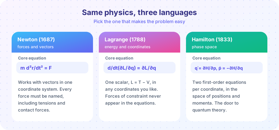
Three formulations, one physics
| Newton | Lagrange | Hamilton | |
|---|---|---|---|
| Variables | position vectors | generalized coordinates q, velocities q̇ |
coordinates q and momenta p |
| Core object | force F |
scalar L = T − V |
scalar H = T + V (often) |
| Equation order | second order | second order | first order, twice as many |
| Constraint forces | must be solved | disappear | disappear |
| Strength | simple problems, intuition | constraints, any coordinates | symmetry, phase space, quantum theory |
All three give identical trajectories whenever they apply. The differences are about convenience and about what generalizes to new physics.
A problem that rewards energy thinking
Take a bead on a hoop of radius R rotating at constant ω about its vertical diameter, with θ measured from the bottom. Chapter 4 derives the equation, and the demonstration below only needs the result:
θ̈ = ω² sinθ cosθ − (g/R) sinθ
The bottom θ = 0 is always an equilibrium. When ω is small it is stable. Above the critical value ω_c = √(g/R) it becomes unstable and the bead prefers an angle with cos θ = g/(R ω²).
Press Run (or Ctrl + Enter) to see the result here.
Program input · what you'd type while the program runs
Type the answers before you press Run, one per line. Each time the program reads a line (with input()), it gets the next line from this box.
Below the critical speed the bead just wiggles about θ = 0 (a tiny line). Above it, the bead swings away and oscillates about the new equilibrium. The reason is energy: spinning makes outward positions cheaper in the effective potential (chapter 5). You can predict the new angle with one line of algebra.
Press Run (or Ctrl + Enter) to see the result here.
Program input · what you'd type while the program runs
Type the answers before you press Run, one per line. Each time the program reads a line (with input()), it gets the next line from this box.
The angle grows from zero as soon as ω passes ω_c and approaches 90° (the bead at hoop height) at high speeds: an example of a bifurcation that Newton's vector method hides inside the force bookkeeping.
Counting the work: Newton versus Lagrange
Numbers make the advantage concrete. Take a bead of mass 0.1 kg on a vertical hoop of radius 0.5 m that spins about its vertical axis at a steady rate. In Newton's method you must choose axes, write the radial, tangential and out-of-plane components of F = ma, and carry two unknown constraint forces (the normal force from the wire has two independent components) through the algebra, only to eliminate them at the end. In the Lagrangian method you write T and V in the single coordinate θ, differentiate once, and the constraint forces never appear. One coordinate gives one equation.
The result of that single equation is that the bead sits at θ = 0 (the bottom) unless the hoop spins faster than the critical rate ω_c = √(g/R). For R = 0.5 m and g = 9.81 m/s² this is √19.62 ≈ 4.43 rad/s, about 0.70 revolutions per second. Spin it at ω = 6 rad/s and the bottom becomes unstable: the bead climbs to cos θ = g/(ω²R) = 9.81/18 ≈ 0.545, that is θ ≈ 57°. Chapter 4 derives this properly; for now notice how little algebra the energy viewpoint needs.
Who built this, and why it matters
Pierre de Maupertuis (1744) proposed that nature minimizes a quantity he called action, and Leonhard Euler turned the idea into a precise mathematical method in the same year. Joseph-Louis Lagrange, aged 19, sent Euler his improved method in 1755, built on it for decades and published Mécanique analytique in 1788, famous for containing no diagrams at all: everything followed from analysis. Jean le Rond d'Alembert had in 1743 shown how to turn dynamics into statics by adding an "inertia force", and the principle of virtual work (Johann Bernoulli, 1717) supplied the rest. William Rowan Hamilton (1833-35) then recast the theory in terms of momenta, which is the formulation closest to quantum mechanics. Each step kept Newton's physics intact and changed only the bookkeeping.
What you gain, and what you do not
You gain generality (one method for pendulums, planets and fields), a direct line to conservation laws (chapter 5), and equations that keep the same form in every coordinate system. You do not gain new predictions for ordinary mechanics: if a Lagrangian problem and a Newtonian problem describe the same system, they must give identical motion. Treat the Lagrangian approach as a better language rather than a rival theory.
Common misconceptions
"Lagrangian mechanics is different physics." No. Whenever both apply they give the same answers; Lagrange is a reformulation, not a new law.
"Constraint forces vanish." They exist and are often needed (a rope must hold!). The method just does not need them to find the motion, and you can recover them afterwards with Lagrange multipliers.
Check your understanding
Quick check · 4 questions
of 4 answered You scored / 4 · perfect!
-
1. Why do constraint forces not appear in Lagrange's equations?
Constraint forces are perpendicular to the allowed displacements, so they contribute no virtual work. -
2. How many Lagrange equations does a bead on a hoop need?
The system has one degree of freedom, so one generalized coordinate and one equation. -
3. For the rotating hoop, what happens when ω exceeds √(g/R)?
The effective restoring force changes sign near θ = 0, and a new equilibrium appears at cos θ = g/(Rω²). -
4. Which formulation uses positions and momenta as independent variables?
Hamilton's equations treat q and p as independent coordinates on phase space.
Summary
- Constraints force you to solve for unknown forces in Newton's method; Lagrange avoids them.
- Euler, Lagrange, Hamilton and Jacobi built the framework between 1740 and 1840.
- Newton, Lagrange and Hamilton give the same trajectories; they differ in convenience.
- A rotating hoop shows how a simple energy-based equation reveals a change of equilibrium.
Track your progress
Create a free account to tick off lessons and pick up where you left off on any device.
of Classical Mechanics: Lagrangian and Hamiltonian lessons completed