


















Lesson 40 of 44 · Projects and Practice
Project: Symplectic Integrators
Compare explicit Euler, symplectic Euler, leapfrog and RK4 on the oscillator and a Kepler orbit, and see why preserving phase-space area keeps energy bounded.
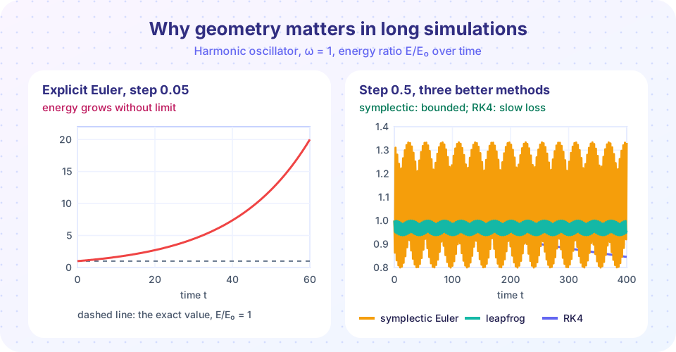
Hamiltonian systems have a rigid geometry: their flow keeps phase-space area (Liouville) and, more generally, preserves the symplectic structure. A numerical method that ignores this geometry can look accurate for a short run and still go badly wrong in a long one, with energy slowly leaking away or growing without limit. A method that respects the geometry, a symplectic integrator, does something different: it makes errors, but they stay bounded and the energy hovers around its true value forever.
This project lets you see it. You will implement four methods in a few lines each, measure what they do to phase-space area in one step, and run them over hundreds of Kepler orbits.
What you will learn
- How four standard one-step methods are written for
q̇ = p,ṗ = −V'(q). - Why explicit Euler multiplies phase-space area by
1 + ω²Δt²per step. - Why symplectic methods keep energy error bounded.
- How to choose a method for a long orbit calculation.
Key terms
Integrator: a rule that advances (q, p) by a step Δt.
Symplectic: the one-step map is a canonical transformation, so it preserves phase-space area (and the Poisson bracket).
Leapfrog (Störmer-Verlet): half kick, full drift, half kick.
Shadow Hamiltonian: a nearby Hamiltonian that a symplectic integrator conserves almost exactly.
Four methods
All four advance q̇ = p/m, ṗ = F(q) = −V'(q) (take m = 1). Write a = F(q).
| Method | Update | Order |
|---|---|---|
| Explicit Euler | q' = q + Δt p, p' = p + Δt F(q) |
1 |
| Symplectic Euler | p' = p + Δt F(q), q' = q + Δt p' |
1 |
| Leapfrog | p½ = p + ½Δt F(q), q' = q + Δt p½, p' = p½ + ½Δt F(q') |
2 |
| RK4 | the classical four-stage Runge-Kutta scheme | 4 |
The difference between the first two is only which p you use in the position update: the old one or the new one. That tiny change flips the geometry.
What happens to area in one step
For the oscillator F = −ω²q every method is a linear map (q, p) → (q', p'), so its effect on area is the determinant of the 2 × 2 matrix.
- Explicit Euler:
det = 1 + ω²Δt². Area grows every step, and the energy grows by the same factor,E' = (1 + ω²Δt²)E. - Symplectic Euler and leapfrog:
det = 1exactly. They are canonical transformations. - RK4:
detis slightly less than 1 (by aboutΔt⁶terms): high accuracy, but not area preserving, so over very long times energy decays slowly.
A symplectic method exactly solves the motion of a slightly different Hamiltonian H̃ = H + O(Δt²) (the shadow Hamiltonian). Since H̃ is conserved exactly, H can only oscillate near it. This is why the energy error of leapfrog does not grow, even over millions of steps, as long as the step is small enough for the shadow Hamiltonian to exist.
For long simulations of planetary systems, molecules, or plasma, symplectic methods are the default choice. Use RK4 (or adaptive higher-order methods) when you need small error over a short time or when the system is dissipative.
Common misconceptions
- "Higher order is always better." RK4 is far more accurate per step, but over very long runs its slow energy loss can beat a second-order symplectic method that never drifts.
- "A symplectic method conserves energy exactly." It conserves a nearby Hamiltonian; the true energy oscillates by
O(Δt²). If the step is too large the picture breaks down. - "Leapfrog and Euler are nearly the same, so one can use either." Explicit Euler grows the energy exponentially, even for a harmonic oscillator.
Try it
The first TryIt implements the four methods for the oscillator (ω = 1, m = 1) and measures two things: the determinant of the one-step map (what each step does to area) and the energy ratio E/E₀ after 1000 steps of Δt = 0.1 (t = 100) starting from q = 1, p = 0. All numbers are computed by the code.
Press Run (or Ctrl + Enter) to see the result here.
Program input · what you'd type while the program runs
Type the answers before you press Run, one per line. Each time the program reads a line (with input()), it gets the next line from this box.
The second TryIt runs a Kepler orbit in units where μ = k = 1: eccentricity e = 0.6, semi-major axis a = 1 (period 2π), starting at closest approach (0.4, 0) with velocity (0, 2). It integrates with leapfrog, symplectic Euler and RK4 at the same step (Δt = 0.02) for 300 orbits and plots the energy error and how the orbit's direction of closest approach (the Runge-Lenz angle) turns. The true orbit has a fixed perihelion direction, so any turning is numerical error.
Press Run (or Ctrl + Enter) to see the result here.
Program input · what you'd type while the program runs
Type the answers before you press Run, one per line. Each time the program reads a line (with input()), it gets the next line from this box.
Reading the results honestly
In the run above (Δt = 0.02, 300 orbits), all three methods behave well, and the comparison is more interesting than "symplectic wins". The first TryIt shows the clean picture: explicit Euler's energy grows by a factor of about 21,000 over 1000 steps, while symplectic Euler and leapfrog stay within a few percent of the truth, and RK4 stays very close at this small step. The Kepler run shows the trade-offs:
- Leapfrog: the energy error is bounded (it oscillates, it does not grow), but the orbit's perihelion slowly turns: a numerical precession of tens of degrees after 300 orbits. The method preserves the geometry but not the exact shape.
- Symplectic Euler is first order: its energy error is bounded but swings about twenty times more at close approach.
- RK4 has a very small error here, but it has a steady drift in
E(a slow monotone trend). Run it for far more orbits, or with a larger step, and that drift eventually overtakes the bounded error of the symplectic methods.
Change dt to 0.05 and orbits to 1000 in the code and watch what happens to the three energy curves. The right method depends on the step size and the length of the run: this is the kind of experiment you should always do before trusting a long simulation.
Check your understanding
Quick check · 5 questions
of 5 answered You scored / 5 · perfect!
-
1. What is the determinant of one step of explicit Euler for the oscillator?
Each step multiplies area (and energy) by 1 + ω²Δt², so both grow without bound. -
2. Which pair of methods is symplectic?
Both have a one-step map with determinant exactly 1 for the oscillator, and they are canonical transformations in general. -
3. What does a symplectic integrator conserve almost exactly?
It solves a nearby Hamiltonian exactly, so the true energy oscillates but does not drift. -
4. In leapfrog, the position is updated with which momentum?
Half kick p½ = p + ½Δt F, then drift q' = q + Δt p½, then a second half kick. -
5. For a dissipative system (friction), what is a good choice?
Friction destroys the symplectic structure; accuracy per step matters more.
Summary
- Explicit Euler multiplies phase-space area (and energy) by
1 + ω²Δt²each step; symplectic Euler and leapfrog preserve it. - Symplectic methods conserve a shadow Hamiltonian, so energy errors stay bounded over very long runs.
- RK4 is more accurate per step but slowly loses energy; use symplectic methods for long Hamiltonian simulations.
Next: Practice problem set
Track your progress
Create a free account to tick off lessons and pick up where you left off on any device.
of Classical Mechanics: Lagrangian and Hamiltonian lessons completed