


















Lesson 4 of 44 · Getting Started
Generalized Coordinates and Degrees of Freedom
Learn how to count degrees of freedom, choose generalized coordinates for pendulums and other systems, and write kinetic energy in those coordinates, with symbolic Python.
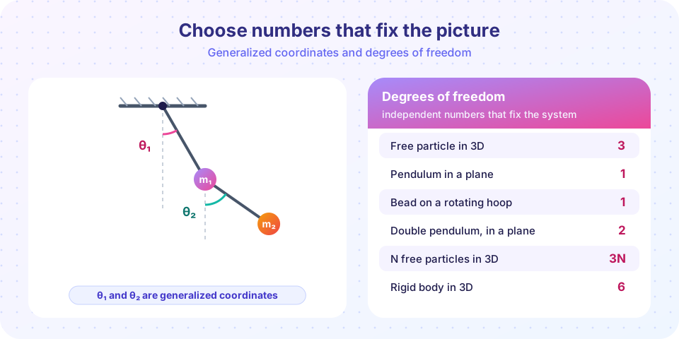
The first decision in any Lagrangian problem is the choice of coordinates. In Newton's method you use the Cartesian axes by default, and constraints are added as forces. In Lagrange's method you choose coordinates that already respect the constraints. A pendulum bob is described by one angle instead of two coordinates plus a rod force. This lesson shows how to count, choose and use such coordinates.
What you will learn
- What a degree of freedom is and how to count them with
n = 3N − k. - The difference between holonomic and non-holonomic constraints.
- How to write positions and kinetic energy in generalized coordinates.
- What makes a good choice of coordinates.
Key terms
A degree of freedom is an independent way the system can move. Generalized coordinates q₁ … qₙ are n independent variables that fix every position. A holonomic constraint is an equation f(r₁, …, r_N, t) = 0. Configuration space is the n-dimensional space of all q values.
Counting degrees of freedom
N free particles in three dimensions need 3N numbers. Each holonomic constraint removes one:
n = 3N − k
Examples.
- A bead on a circular wire in a plane:
N = 1, three coordinates butz = 0andx² + y² = R², sok = 2andn = 1. - A rigid rod of length
ljoining two particles:N = 2, one constraint|r₁ − r₂| = l, son = 6 − 1 = 5. - A rigid body (many particles with fixed distances) has
n = 6: three for position, three for orientation. - A double pendulum in a plane:
N = 2particles in 2D give 4 numbers, two rod constraints remove 2, son = 2.
Choosing generalized coordinates
Generalized coordinates are any n independent quantities that fix the configuration: angles, lengths, distances along a curve, even amplitudes. They need not have the dimension of length. Each position is written as a function of them:
rᵢ = rᵢ(q₁, …, qₙ, t)
For the double pendulum, put the origin at the pivot, x to the right and y up, and measure both angles from the downward vertical:
x₁ = l₁ sin θ₁            y₁ = −l₁ cos θ₁
x₂ = l₁ sin θ₁ + l₂ sin θ₂ y₂ = −l₁ cos θ₁ − l₂ cos θ₂
Velocities follow from the chain rule: ṙᵢ = Σⱼ (∂rᵢ/∂qⱼ) q̇ⱼ + ∂rᵢ/∂t. Substituting in T = Σ ½ mᵢ ṙᵢ² gives kinetic energy as a quadratic form in the generalized velocities, with coefficients that may depend on q.
Good choices share three traits: they match the symmetry (angles for rotation, distance along a track), they are all independent, and they make T and V short. If a problem has a conserved quantity, a coordinate that does not appear in L (a "cyclic" coordinate, chapter 5) gives a free first integral.
Not every constraint is holonomic
- Inequality constraints only keep a particle on one side: a ball on a sphere can leave the surface. The constraint holds only while contact lasts.
- Non-holonomic constraints involve velocities that cannot be integrated into a relation between coordinates alone: a skate blade or a rolling coin must roll without slipping sideways, but it can reach any position and orientation. The count
3N − kno longer holds. - Time-dependent (rheonomic) constraints such as a rotating hoop have
tin the constraint equation. They are holonomic but makeTdepend on time.
This course concentrates on holonomic systems; the others appear as warnings in later chapters.
Worked counts of degrees of freedom
The rule is n = 3N − k for N particles with k independent holonomic constraints. Try it on real systems.
| System | N | Constraints | n | Natural coordinates |
|---|---|---|---|---|
| Bead on a straight wire | 1 | 2 | 1 | distance along the wire s |
| Planar pendulum | 1 | 2 (plane, fixed length) | 1 | angle θ |
| Spherical pendulum | 1 | 1 (fixed length) | 2 | θ, φ |
| Planar double pendulum | 2 | 4 (plane, two lengths) | 2 | θ₁, θ₂ |
| Two masses on a rigid rod (3D) | 2 | 1 | 5 | center (3) plus two angles |
| Rigid body, 3+ non-collinear points | N | 3N − 6 | 6 | 3 position plus 3 orientation |
The last row deserves a remark. A rigid body contains countless particles, but all its internal distances are fixed. Once three non-collinear points are placed, every other point is determined, and the three points have 9 coordinates tied by 3 distance constraints, leaving 9 − 3 = 6: three numbers for where the body is and three for how it is turned.
A number-checking exercise
Imagine a double pendulum with rods l₁ = 1 m and l₂ = 0.5 m. Using (θ₁, θ₂), the second bob is at r₂ = (l₁ sin θ₁ + l₂ sin θ₂, −l₁ cos θ₁ − l₂ cos θ₂). At θ₁ = θ₂ = 0 (hanging straight down) it is at (0, −1.5); at θ₁ = 90°, θ₂ = 0 it is at (1, −0.5). Both points are at most 1.5 m from the pivot, which is what the constraints require. If you asked for a bob position 2 m from the pivot, no (θ₁, θ₂) exists: the reachable region is smaller than the plane, so the map from angles to the workspace is not onto.
Why not just use x and y?
You could keep Cartesian coordinates and add each constraint as an equation, but then the equations are no longer independent and you must carry constraint forces. Choosing n independent coordinates removes the problem at the root. A good choice also exposes symmetry: if a coordinate does not appear in L, its momentum is conserved (chapter 5), and this is only visible in coordinates adapted to the problem (an angle for rotational symmetry, not x and y).
The term holonomic comes from Heinrich Hertz (1894), meaning "whole" or "integral": a constraint that can be integrated down to a relation among coordinates. A rolling disk is the standard non-example. Its rolling condition relates velocities and cannot be integrated, so the disk can reach any position and orientation even though its instantaneous motion is restricted.
Common misconceptions
"A generalized coordinate must be a length." No: angles, areas or any quantity that labels the configuration will do. The conjugate generalized momentum then has matching dimensions (angular momentum for an angle).
"More coordinates is safer." Extra coordinates reintroduce the constraints you wanted to avoid. Use exactly n independent ones.
Try it
Let a computer algebra system do the substitution for the double pendulum. It builds the positions, differentiates, and simplifies the kinetic energy.
Press Run (or Ctrl + Enter) to see the result here.
Program input · what you'd type while the program runs
Type the answers before you press Run, one per line. Each time the program reads a line (with input()), it gets the next line from this box.
Next, see what two angles do. Every pair (θ₁, θ₂) is one point of configuration space, and it corresponds to one position of the lower bob. Plotting a grid of pairs shows the reachable region (an annulus) and also that many angle pairs give the same tip position.
Press Run (or Ctrl + Enter) to see the result here.
Program input · what you'd type while the program runs
Type the answers before you press Run, one per line. Each time the program reads a line (with input()), it gets the next line from this box.
Check your understanding
Quick check · 5 questions
of 5 answered You scored / 5 · perfect!
-
1. How many degrees of freedom does a rigid body in three dimensions have?
Three coordinates fix the position of a reference point and three angles fix the orientation. -
2. A bead slides on a fixed circular wire in a plane. How many generalized coordinates are needed?
One angle around the circle fixes the bead completely. -
3. Two particles in 3D are joined by a rigid massless rod. What is n?
3N = 6 numbers, minus one constraint |r₁ − r₂| = l, gives 5. -
4. Which constraint is non-holonomic?
The no-slip condition restricts velocities but cannot be integrated into a relation between coordinates alone. -
5. Why does the kinetic energy of a double pendulum contain cos(θ₁ − θ₂)?
|v₂|² contains the dot product of the two rod velocities, which brings in cos(θ₁ − θ₂).
Summary
n = 3N − kcounts the degrees of freedom of a system withkholonomic constraints.- Generalized coordinates are exactly
nindependent variables (angles, lengths, anything) that fix the configuration. - Write
rᵢ(q, t), differentiate with the chain rule and substitute intoTto get kinetic energy in generalized coordinates. - Inequality, velocity-dependent and time-dependent constraints need extra care.
Next: Chapter 1 Review
Track your progress
Create a free account to tick off lessons and pick up where you left off on any device.
of Classical Mechanics: Lagrangian and Hamiltonian lessons completed