Derive the double pendulum's equations with sympy, simulate it, check energy conservation and measure how fast two nearly identical starts drift apart.
Two rods and two masses: it hardly gets simpler as a mechanical system, and yet the double pendulum is the classic example of chaos. Two runs that start almost identically stay together for a while, then separate completely. This project takes you from the Lagrangian to the equations, to a numerical solution, to a measurement of how quickly predictions fail.
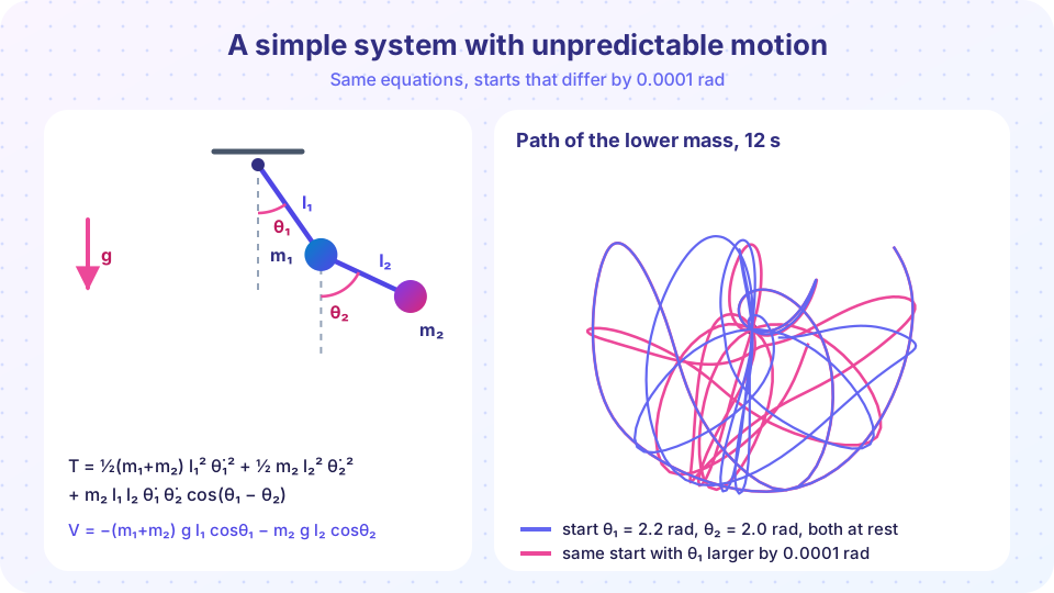
Caption: left, the setup and the Lagrangian pieces; right, the path of the lower mass for two starts that differ by 0.0001 rad, which separate after a few seconds.
Differentiate, form T = ½m₁(ẋ₁² + ẏ₁²) + ½m₂(ẋ₂² + ẏ₂²) and V = m₁gy₁ + m₂gy₂, and simplify:
Text
T = ½(m₁ + m₂) l₁² θ̇₁² + ½ m₂ l₂² θ̇₂² + m₂ l₁ l₂ θ̇₁ θ̇₂ cos(θ₁ − θ₂)
V = −(m₁ + m₂) g l₁ cosθ₁ − m₂ g l₂ cosθ₂
Notice the cross term in T: the two angles are coupled through their velocities, not only through the potential. That is why the motion is complicated. Since L has no explicit time dependence, the energy E = T + V is conserved. There is no cyclic coordinate and no second conserved quantity, so the system is not integrable: you cannot reduce the problem to quadratures.
The Euler-Lagrange equations give two coupled second-order equations. For the equal-mass, equal-length case they can be written as M(θ) θ̈ = F(θ, θ̇) with
Text
M = m l² [[2, cos(θ₁ − θ₂)], [cos(θ₁ − θ₂), 1]]
F₁ = −m l² θ̇₂² sin(θ₁ − θ₂) − 2 m g l sinθ₁
F₂ =  m l² θ̇₁² sin(θ₁ − θ₂) − m g l sinθ₂
Solving the 2 × 2 system gives the accelerations; the sympy code does this for general masses and lengths.
"Chaotic means random." The equations are completely deterministic. The unpredictability comes from magnifying tiny differences, not from randomness.
"A better computer solves it." The error in a chaotic simulation grows exponentially. Improving precision by a factor of 10⁶ extends the prediction horizon by a fixed amount of time, roughly ln(10⁶)/λ, not indefinitely.
"Chaos means no conservation law." Energy is exactly conserved here; chaos limits what you can predict about the configuration, not the energy.
The first TryIt derives the equations with sympy from the Lagrangian (general masses and lengths), then integrates them for m₁ = m₂ = 1 kg, l₁ = l₂ = 1 m, starting at rest at θ₁ = 2.2 rad, θ₂ = 2.0 rad. It checks the energy and compares the sympy accelerations with a closed-form expression at many points of the trajectory (this closed form is the one used in the interactive demo below). Deriving takes a few seconds, which is normal for symbolic algebra.
Python
From L to the double pendulum
import numpy as np
import sympy as sp
from scipy.integrate import solve_ivp
import matplotlib.pyplot as plt
plt.rcParams.update({"figure.facecolor":"#faf5ff","axes.facecolor":"#ffffff","axes.edgecolor":"#c7d2fe","axes.spines.top":False,"axes.spines.right":False,"axes.grid":True,"grid.color":"#eef2ff","axes.prop_cycle": plt.cycler(color=["#6366f1","#ec4899","#f59e0b","#14b8a6","#38bdf8"]),"font.size":12})
t = sp.symbols("t")
m1, m2, l1, l2, g = sp.symbols("m1 m2 l1 l2 g", positive=True)
a, b = sp.Function("theta1")(t), sp.Function("theta2")(t)
T = sp.Rational(1,2)*(m1 + m2)* l1**2* a.diff(t)**2+ sp.Rational(1,2)* m2 * l2**2* b.diff(t)**2 \
+ m2 * l1 * l2 * a.diff(t)* b.diff(t)* sp.cos(a - b)
V =-(m1 + m2)* g * l1 * sp.cos(a)- m2 * g * l2 * sp.cos(b)
L = T - V
qs, qd, qdd =[a, b],[a.diff(t), b.diff(t)],[a.diff(t,2), b.diff(t,2)]
eqs =[sp.diff(sp.diff(L, v), t)- sp.diff(L, q)for q, v inzip(qs, qd)]
acc = sp.solve(eqs, qdd,dict=True)[0]
Q, W = sp.symbols("Q0:2"), sp.symbols("W0:2")
swap ={a: Q[0], b: Q[1], qd[0]: W[0], qd[1]: W[1]}
num ={m1:1.0, m2:1.0, l1:1.0, l2:1.0, g:9.81}
acc_fun = sp.lambdify([*Q,*W],[acc[qdd[0]].subs(swap).subs(num), acc[qdd[1]].subs(swap).subs(num)],"numpy")
rhs =lambda tt, y:[y[2], y[3],*acc_fun(*y)]
sol = solve_ivp(rhs,(0,10),[2.2,2.0,0.0,0.0], t_eval=np.linspace(0,10,1000), rtol=1e-10, atol=1e-12)
th1, th2, w1, w2 = sol.y
E =0.5*2* w1**2+0.5* w2**2+ w1 * w2 * np.cos(th1 - th2)-2*9.81* np.cos(th1)-9.81* np.cos(th2)print("energy E varies by",f"{E.max()- E.min():.2e} J over 10 s (E = {E[0]:.4f} J)")defclosed_form(t1, t2, v1, v2, g=9.81):
d = t1 - t2
den =3- np.cos(2* d)
A1 =(-3* g * np.sin(t1)- g * np.sin(t1 -2* t2)-2* np.sin(d)*(v2**2+ v1**2* np.cos(d)))/ den
A2 =(2* np.sin(d)*(2* v1**2+2* g * np.cos(t1)+ v2**2* np.cos(d)))/ den
return A1, A2
worst =0.0for i inrange(0,1000,20):
s = acc_fun(th1[i], th2[i], w1[i], w2[i])
c = closed_form(th1[i], th2[i], w1[i], w2[i])
worst =max(worst,abs(s[0]- c[0]),abs(s[1]- c[1]))print("largest difference between sympy and the closed form:",f"{worst:.1e} rad/s^2")
x2, y2 = np.sin(th1)+ np.sin(th2),-np.cos(th1)- np.cos(th2)
plt.figure(figsize=(6,5))
plt.scatter(x2, y2, c=sol.t, s=6, cmap="plasma")
plt.colorbar(label="time (s)")
plt.plot([0],[0],"ko")
plt.gca().set_aspect("equal")
plt.xlabel("x of the lower mass (m)")
plt.ylabel("y of the lower mass (m)")
plt.title("Path of the lower mass, 10 s")
plt.tight_layout()
plt.show()
Press Run (or Ctrl + Enter) to see the result here.
Program input · what you'd type while the program runs
Type the answers before you press Run, one per line. Each time the program reads a line (with input()), it gets the next line from this box.
The second TryIt measures the chaos. It integrates two runs whose initial θ₁ differ by 10⁻⁸ rad and plots the distance between them, d = √(Δθ₁² + Δθ₂²), on a logarithmic axis. In the exponential-growth region the slope is an estimate of the Lyapunov exponent λ. This exponent depends on the starting point and energy, and a single trajectory gives only a rough estimate.
Python
How fast do nearby starts separate?
import numpy as np
from scipy.integrate import solve_ivp
import matplotlib.pyplot as plt
plt.rcParams.update({"figure.facecolor":"#faf5ff","axes.facecolor":"#ffffff","axes.edgecolor":"#c7d2fe","axes.spines.top":False,"axes.spines.right":False,"axes.grid":True,"grid.color":"#eef2ff","axes.prop_cycle": plt.cycler(color=["#6366f1","#ec4899","#f59e0b","#14b8a6","#38bdf8"]),"font.size":12})
g =9.81defrhs(t, s):
t1, t2, w1, w2 = s
d = t1 - t2
den =3- np.cos(2* d)
a1 =(-3* g * np.sin(t1)- g * np.sin(t1 -2* t2)-2* np.sin(d)*(w2**2+ w1**2* np.cos(d)))/ den
a2 =(2* np.sin(d)*(2* w1**2+2* g * np.cos(t1)+ w2**2* np.cos(d)))/ den
return[w1, w2, a1, a2]
delta =1e-8
t = np.linspace(0,25,5000)
A = solve_ivp(rhs,(0,25),[2.2,2.0,0,0], t_eval=t, rtol=1e-12, atol=1e-13).y
B = solve_ivp(rhs,(0,25),[2.2+ delta,2.0,0,0], t_eval=t, rtol=1e-12, atol=1e-13).y
d = np.hypot(A[0]- B[0], A[1]- B[1])
grow =(d >1e-7)&(d <1e-1)
lam = np.polyfit(t[grow], np.log(d[grow]),1)[0]print(f"estimated Lyapunov exponent: {lam:.2f} per second")print(f"an error of {delta:g} rad reaches 1 rad after about {np.log(1/ delta)/ lam:.1f} s")
plt.figure(figsize=(8,4.4))
plt.semilogy(t, d +1e-16, linewidth=2.5)
plt.semilogy(t[grow], np.exp(np.polyval(np.polyfit(t[grow], np.log(d[grow]),1), t[grow])),"--", linewidth=2.5, color="#ec4899", label=f"exponential fit, λ ≈ {lam:.2f} s⁻¹")
plt.axhline(1, color="#94a3b8", linewidth=1)
plt.annotate("saturation: the two runs\nare now unrelated", xy=(21,1.2), xytext=(8,3e-4), arrowprops=dict(arrowstyle="->", color="#475569"))
plt.xlabel("time (s)")
plt.ylabel("distance between the runs (rad)")
plt.title("Sensitive dependence on initial conditions")
plt.legend(loc="lower right")
plt.tight_layout()
plt.show()
Press Run (or Ctrl + Enter) to see the result here.
Program input · what you'd type while the program runs
Type the answers before you press Run, one per line. Each time the program reads a line (with input()), it gets the next line from this box.
The third TryIt is the double pendulum as a live animation (equal masses and lengths, g = 9.81 m/s², fourth-order Runge-Kutta). Choose the starting angles, press Restart, and switch on the pink twin, a second pendulum whose θ₁ is larger by 0.001 rad. At first you see one pendulum; later the twin goes its own way. It is a simulation of the model equations, not a recording of a real pendulum.