


















Lesson 28 of 44 · Hamiltonian Mechanics
Poisson Brackets and Canonical Transformations
Use the Poisson bracket to compute time evolution and conserved quantities, then learn canonical transformations, generating functions and action-angle variables.
Hamilton's equations treat q and p almost symmetrically, and there is a compact bookkeeping device that makes this precise: the Poisson bracket. It answers the question "how does any quantity f(q, p, t) change in time?" with one formula, gives a one-line test for conserved quantities, and sets up the algebra that quantum mechanics later promotes to commutators.
The second half of the lesson asks which changes of variables (q, p) → (Q, P) keep Hamilton's equations looking the same. These canonical transformations are what you use to simplify a problem until it is trivial, as in the action-angle variables of the harmonic oscillator.
What you will learn
- How to compute and use
{f, g}and its four rules. - How to test whether a quantity is conserved with
{f, H}. - What makes a transformation canonical, and how generating functions produce one.
- How action-angle variables solve the harmonic oscillator.
Key terms
Poisson bracket: {f, g} = Σᵢ (∂f/∂qᵢ ∂g/∂pᵢ − ∂f/∂pᵢ ∂g/∂qᵢ).
Canonical transformation: a change of variables (q, p) → (Q, P) that keeps {Qᵢ, Pⱼ} = δᵢⱼ and the form of Hamilton's equations.
Generating function: a single function whose derivatives give the whole transformation.
Action-angle variables: canonical variables in which H depends only on the action P.
The Poisson bracket
For two functions f(q, p) and g(q, p) of a system with n degrees of freedom:
{f, g} = Σᵢ ( ∂f/∂qᵢ · ∂g/∂pᵢ − ∂f/∂pᵢ · ∂g/∂qᵢ )
(Some books use the opposite sign; this lesson uses the convention that gives ḟ = {f, H}.)
Four rules make it easy to use:
| Rule | Statement |
|---|---|
| Antisymmetry | {f, g} = −{g, f}, so {f, f} = 0 |
| Linearity | {af + bg, h} = a{f, h} + b{g, h} |
| Leibniz (product rule) | {fg, h} = f{g, h} + {f, h}g |
| Jacobi identity | {f, {g, h}} + {g, {h, f}} + {h, {f, g}} = 0 |
The fundamental brackets are the ones from which everything else follows:
{qᵢ, pⱼ} = δᵢⱼ, {qᵢ, qⱼ} = 0, {pᵢ, pⱼ} = 0
Time evolution
Let f(q, p, t) be any observable. By the chain rule and Hamilton's equations:
df/dt = ∂f/∂t + Σ (∂f/∂q · q̇ + ∂f/∂p · ṗ)
      = ∂f/∂t + Σ (∂f/∂q · ∂H/∂p − ∂f/∂p · ∂H/∂q)
      = ∂f/∂t + {f, H}
Hamilton's equations are the special cases q̇ = {q, H} and ṗ = {p, H}. A quantity with no explicit time dependence is conserved if and only if {f, H} = 0. That includes H itself: {H, H} = 0.
Poisson's theorem
If f and g are both conserved, then so is {f, g}. This follows from the Jacobi identity: if {f, H} = 0 and {g, H} = 0 then {{f, g}, H} = −{{g, H}, f} − {{H, f}, g} = 0. Sometimes the new constant is trivial, but sometimes it is a surprise (the Runge-Lenz vector of the Kepler problem generates more constants this way).
Angular momentum
For L = r × p the brackets are
{Lₓ, L_y} = L_z, {L_y, L_z} = Lₓ, {L_z, Lₓ} = L_y
and {L², L_z} = 0. Two components of angular momentum do not Poisson-commute, so they cannot both be used as "momenta" in the same set of canonical coordinates. In quantum mechanics the same algebra appears with [Lₓ, L_y] = iħL_z. Dirac's rule: replace { , } by (1/iħ)[ , ].
Canonical transformations
A transformation Qᵢ(q, p, t), Pᵢ(q, p, t) is canonical if the new variables satisfy the fundamental brackets, computed in the old variables:
{Qᵢ, Pⱼ} = δᵢⱼ, {Qᵢ, Qⱼ} = 0, {Pᵢ, Pⱼ} = 0
Then there is a new Hamiltonian K(Q, P, t) such that Q̇ = ∂K/∂P and Ṗ = −∂K/∂Q. The brackets are the same in every canonical set of variables, which is why ḟ = {f, H} is true in all of them.
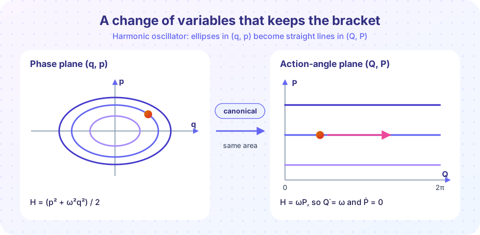
For one degree of freedom this condition says ∂(Q, P)/∂(q, p) = 1: the transformation preserves areas (it has Jacobian determinant 1). That is the same property Liouville gave the Hamiltonian flow. In fact the flow from time 0 to time t is itself a canonical transformation.
Generating functions
You rarely guess a canonical transformation. Instead you choose a generating function, and it produces one:
| Type | Depends on | Relations | New Hamiltonian |
|---|---|---|---|
F₁(q, Q, t) |
old q, new Q |
p = ∂F₁/∂q, P = −∂F₁/∂Q |
K = H + ∂F₁/∂t |
F₂(q, P, t) |
old q, new P |
p = ∂F₂/∂q, Q = ∂F₂/∂P |
K = H + ∂F₂/∂t |
Examples.
F₂ = q Pgivesp = P,Q = q: the identity.F₁ = q Qgivesp = Q,P = −q. Coordinates and momenta swap roles, with a sign. The check:{Q, P} = {p, −q} = −{p, q} = 1.- Rescaling
Q = λq,P = p/λis canonical for anyλ ≠ 0;Q = q,P = 2pis not ({Q, P} = 2).
Action-angle variables for the oscillator
For H = p²/2m + ½mω²q² choose F₁(q, Q) = ½mω q² cot Q. Then
p = ∂F₁/∂q = mω q cot Q, P = −∂F₁/∂Q = mω q² / (2 sin²Q)
Solving for q and p:
q = √(2P/(mω)) · sin Q, p = √(2mωP) · cos Q
Substituting into H gives K = H = ωP. Now Q is cyclic, so Ṗ = 0 (P is constant) and Q̇ = ∂K/∂P = ω, so Q = ωt + Q₀. The whole problem is solved by choosing the right variables. P is the action (P = E/ω, the area of the orbit divided by 2π) and Q is the angle that grows steadily from 0 to 2π during one period.
Common misconceptions
- "Any smooth change of variables is allowed." You can use any coordinates in a Lagrangian, but only canonical transformations keep Hamilton's form. For example
P = 2p,Q = qis not canonical. - "
{f, H} = 0meansfis constant even iffdepends explicitly on time." You must include the explicit time term:df/dt = {f, H} + ∂f/∂t. - "The new Hamiltonian
Kis the old one with new names." Equal only for time-independent transformations; time-dependent generating functions add∂F/∂t.
Try it
The first TryIt is a small Poisson-bracket calculator in sympy. It checks the fundamental brackets, the angular momentum algebra, the Jacobi identity, and that L_z commutes with any central-force Hamiltonian p²/2m + V(r). Adding a uniform field breaks that, and the bracket shows which way the angular momentum changes.
Press Run (or Ctrl + Enter) to see the result here.
Program input · what you'd type while the program runs
Type the answers before you press Run, one per line. Each time the program reads a line (with input()), it gets the next line from this box.
The second TryIt checks canonical transformations. It asks whether {Q, P} = 1 for a list of candidates, including the swap, a rescaling, a bad one, and the action-angle transformation (given both in the form Q(q, p) and as the inverse). Seeing 1 means canonical.
Press Run (or Ctrl + Enter) to see the result here.
Program input · what you'd type while the program runs
Type the answers before you press Run, one per line. Each time the program reads a line (with input()), it gets the next line from this box.
The third TryIt uses brackets to solve a problem. The solution of Hamilton's equations can be written as f(t) = f + t{f, H} + (t²/2!){{f, H}, H} + …. For the oscillator (m = 1, k = 4 N/m, so ω = 2 rad/s), take f = x and sum the series. Compare with the exact x(t) = cos 2t for x₀ = 1 m, p₀ = 0. This is the same series as the Taylor series of the cosine, so the comparison shows how fast it converges.
Press Run (or Ctrl + Enter) to see the result here.
Program input · what you'd type while the program runs
Type the answers before you press Run, one per line. Each time the program reads a line (with input()), it gets the next line from this box.
Check your understanding
Quick check · 6 questions
of 6 answered You scored / 6 · perfect!
-
1. For H = p²/2m + V(q), what is {q, H}?
{q, H} = ∂q/∂q · ∂H/∂p = p/m, which is q̇. -
2. A function f(q, p) has no explicit time dependence. When is it conserved?
df/dt = {f, H} + ∂f/∂t, and the second term is zero. -
3. What is {Lₓ, L_y}?
The angular momentum components obey {Lₓ, L_y} = L_z and its cyclic permutations. -
4. Which transformation is canonical?
{3q, p/3} = 1. The first gives 3. For the third, {q², p²} = 4qp, which is not 1. -
5. In action-angle variables the oscillator's Hamiltonian is H = ωP. What is Q̇?
Q̇ = ∂K/∂P = ω. The angle increases at a steady rate and P is constant. -
6. Poisson's theorem says: if f and g are constants of the motion, then...
By the Jacobi identity, {{f, g}, H} = 0 when {f, H} = {g, H} = 0.
Summary
{f, g} = Σ (∂f/∂q ∂g/∂p − ∂f/∂p ∂g/∂q);{q, p} = 1; anddf/dt = {f, H} + ∂f/∂t.fis conserved when{f, H} = 0(no explicit time dependence); the bracket of two constants is a constant.- A canonical transformation keeps the fundamental brackets and can be built from a generating function.
- For the oscillator,
F₁ = ½mωq² cot Qleads toH = ωP, withQ̇ = ωandPconstant.
Next: Chapter 6 review
Track your progress
Create a free account to tick off lessons and pick up where you left off on any device.
of Classical Mechanics: Lagrangian and Hamiltonian lessons completed