


















Lesson 38 of 44 · Projects and Practice
Chapter 9 Overview: Projects and Practice
Plan for the last chapter: build a Lagrangian-to-simulation toolkit, study the chaotic double pendulum and symplectic integrators, then work a problem set.
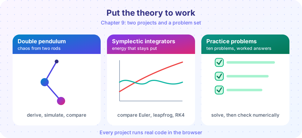
You now have the whole toolkit: Lagrange's equations, conservation laws, Hamilton's equations, orbits, oscillations and rigid bodies. This final chapter puts it to use. Two projects take a system from a Lagrangian to a working simulation and ask what the numbers can and cannot tell you; a problem set tests the methods on new situations; and the end of the chapter holds a glossary, a one-page cheat sheet and suggestions for what to study next.
What you will learn
- How to turn any Lagrangian into a numerical simulation automatically.
- Why the double pendulum is chaotic and what that does to prediction.
- Why some integrators keep energy in order for millions of steps and others do not.
- How to attack unfamiliar problems with a six-step method.
The chapter at a glance
From L to a movie
Project 1: double pendulum
Project 2: integrators
Practice
What each lesson covers
- Project: the double pendulum: derive the equations with sympy, check energy, measure sensitivity to initial conditions.
- Project: symplectic integrators: compare Euler, symplectic Euler, leapfrog and RK4 on the oscillator and a Kepler orbit.
- Practice problem set: ten problems and a six-step method.
- Glossary, cheat sheet and further study.
A reusable tool: from Lagrangian to simulation
The helper in this TryIt does the whole job for the projects. You give it a Lagrangian written with sympy functions q(t), and it forms the Euler-Lagrange equations, solves them for the accelerations, and returns a numerical function f(t, y) that scipy.integrate.solve_ivp can integrate. It is shown on a pendulum (l = 1 m, g = 9.81 m/s², starting at rest at 0.1 rad) and compared with the small-angle answer θ = 0.1 cos(√(g/l) t).
Press Run (or Ctrl + Enter) to see the result here.
Program input · what you'd type while the program runs
Type the answers before you press Run, one per line. Each time the program reads a line (with input()), it gets the next line from this box.
Check your understanding
Quick check · 3 questions
of 3 answered You scored / 3 · perfect!
-
1. What does the helper lagrange_ode compute first?
It differentiates L to form d/dt(∂L/∂q̇) − ∂L/∂q and solves for the accelerations. -
2. Why is a numerical simulation only as good as its checks?
Checking energy and other conserved quantities is the quickest way to catch errors. -
3. What kind of system is the double pendulum?
It has a simple Lagrangian but sensitive dependence on initial conditions at larger energies.
Summary
- A Lagrangian can be turned into a simulation in a few lines with sympy and
solve_ivp. - The two projects test dynamics (chaos) and numerics (energy behavior of integrators).
- Use conserved quantities as checks on every simulation you write.
Track your progress
Create a free account to tick off lessons and pick up where you left off on any device.
of Classical Mechanics: Lagrangian and Hamiltonian lessons completed