


















Lesson 1 of 44 · Getting Started
Course Map: Classical Mechanics from Forces to Action
Start here: who this course is for, what you need to know, how to study it, and a map of all nine chapters from Newton's laws to Hamilton's equations.
Newton's laws tell you how a single particle moves when you know the forces on it. That works wonderfully for a falling apple and badly for a bead sliding on a spinning wire, where the wire pushes on the bead in a way you do not know in advance. In the late 1700s Joseph-Louis Lagrange found a way to skip the unknown forces entirely, and in the 1830s William Rowan Hamilton turned his idea into a second, even more powerful language. This course teaches both.
You will keep the same physics you already know. What changes is the bookkeeping: instead of adding up force vectors, you write down one scalar function built from energies and let a single equation produce the motion. The payoff is huge. The same method handles pendulums, planets, charged particles, spinning tops and, with small changes, quantum mechanics, field theory and general relativity.
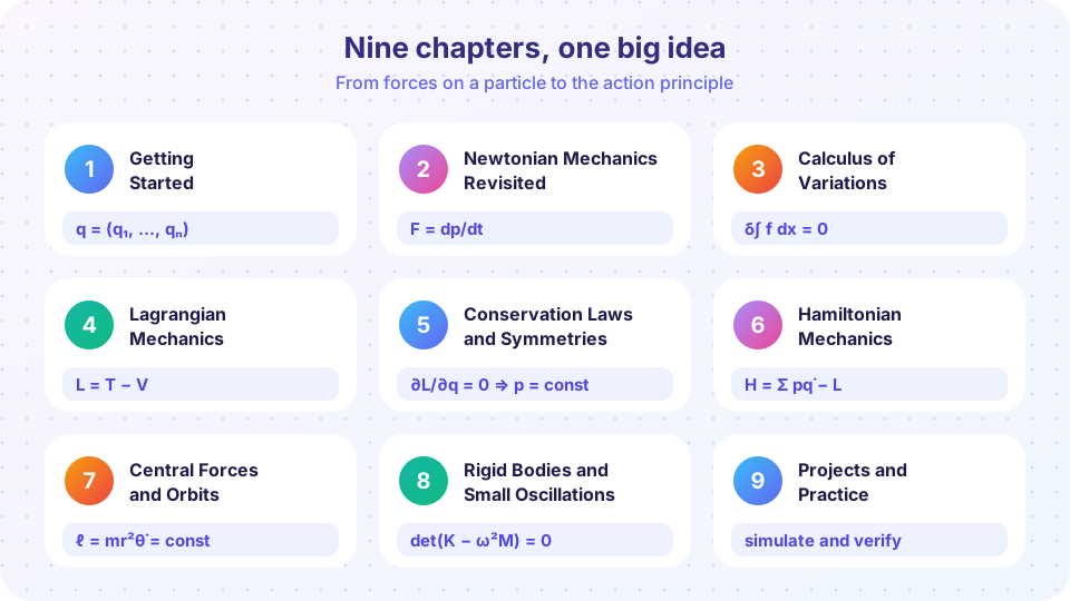
What you will learn
- How to describe a mechanical system with the smallest possible set of coordinates.
- How the calculus of variations finds the path that makes a quantity stationary.
- How to derive and use the Euler-Lagrange equations, and why constraint forces disappear.
- How symmetries produce conservation laws (Noether's theorem) and how Hamilton's equations work in phase space.
- How to solve central-force, rigid-body and small-oscillation problems with these tools, by hand and with code.
Who this course is for
This is an undergraduate-level course for physics, engineering and mathematics students, and for strong high-school students who have finished a first course in mechanics and calculus. It follows the international core taught at university worldwide. You should be comfortable with:
- Newton's three laws, work, kinetic and potential energy, and momentum.
- Differentiation and basic integration, including the chain rule.
- Vectors in two and three dimensions (dot and cross products).
- Simple differential equations such as
ẍ = −ω² x.
You do not need prior knowledge of the calculus of variations, partial differential equations or linear algebra beyond matrices; we introduce them when needed. Dots over letters mean time derivatives: ẋ = dx/dt, ẍ = d²x/dt².
Key terms. Generalized coordinates are independent variables that fix a system's configuration. The Lagrangian L is a scalar function of coordinates, velocities and time, usually T − V. The action is the time integral of L. Phase space is the space of positions and momenta.
The course in five slides
Foundations
Finding the best path
Symmetry and phase space
Applications
Practice
Code runs in your browser
How to study this course
- Read with a pencil. Every derivation is short enough to redo on paper. Do it; the algebra is where the understanding lives.
- Run the code. Each lesson has runnable Python examples. Change a number, predict the result, then run.
- Do the quizzes after the worked examples, not before. They check whether the idea stuck.
- Return to the review lesson at the end of each chapter. The one-page poster is a good thing to copy by hand.
Always draw the system first. A clear picture, with coordinates and angles labelled, prevents most mistakes in the later algebra.
A first taste
Here is the whole method on one example, computed symbolically. We take a pendulum of length l and mass m, write its energies in terms of the angle θ, and let Python apply the Euler-Lagrange equation. Do not worry about the details yet; by the end of chapter 4 you will do this by hand in thirty seconds.
Try it
Press Run (or Ctrl + Enter) to see the result here.
Program input · what you'd type while the program runs
Type the answers before you press Run, one per line. Each time the program reads a line (with input()), it gets the next line from this box.
The second example shows what the equation produces: a phase portrait, a map of every possible motion of the pendulum, with angle on one axis and angular velocity on the other. Closed loops are swings; wavy lines on top and bottom are full rotations. This kind of map is the heart of Hamiltonian mechanics (chapter 6).
Press Run (or Ctrl + Enter) to see the result here.
Program input · what you'd type while the program runs
Type the answers before you press Run, one per line. Each time the program reads a line (with input()), it gets the next line from this box.
Check your understanding
Quick check · 4 questions
of 4 answered You scored / 4 · perfect!
-
1. What is the main practical advantage of the Lagrangian method over Newton's method?
Lagrange's equations use only energies and generalized coordinates, so forces of constraint, such as a rod's tension, never appear. -
2. In this course, what does a dot over a symbol, as in q̇, mean?
A single dot is d/dt and a double dot is d²/dt². -
3. Which pair describes the Lagrangian and Hamiltonian pictures?
L depends on q and q̇, while H lives in phase space with q and p. -
4. In the phase portrait of a pendulum, what do closed loops represent?
A closed loop means the angle and velocity both return to their starting values: a swing.
Summary
- Lagrangian and Hamiltonian mechanics are new bookkeeping for the same physics as Newton's.
- One scalar function,
L = T − V, replaces force vectors, and constraint forces drop out. - The course has nine chapters, from coordinates to projects; each chapter ends with a review poster.
- Run and modify every code example.
Track your progress
Create a free account to tick off lessons and pick up where you left off on any device.
of Classical Mechanics: Lagrangian and Hamiltonian lessons completed