


















Lesson 17 of 44 · Lagrangian Mechanics
From D'Alembert's Principle to Lagrange's Equations
Derive Lagrange's equations from Newton's laws through virtual work and D'Alembert's principle, with generalized forces, dissipation, and symbolic checks in Python.
In the previous chapters you saw that constraint forces are perpendicular to allowed motions. This lesson turns that observation into a derivation. Starting from Newton's second law and the idea of a virtual displacement, we get D'Alembert's principle, and from it Lagrange's equations in a few lines. The result confirms that Lagrangian mechanics is Newtonian mechanics in disguise, and it shows how to include forces that are not derived from a potential.
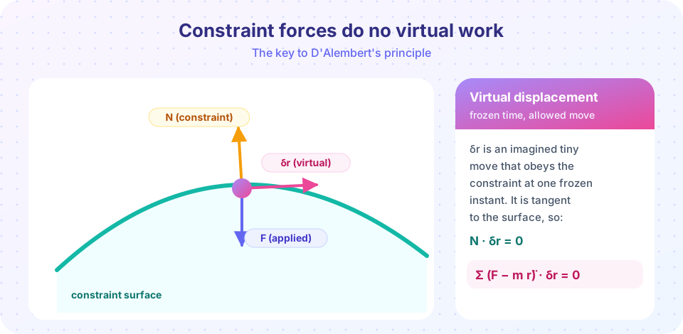
What you will learn
- What a virtual displacement and virtual work are.
- D'Alembert's principle and why constraint forces drop out.
- How to turn it into Lagrange's equations with generalized forces.
- How to handle non-conservative forces such as drag.
Key terms
A virtual displacement δrᵢ is an imagined infinitesimal move consistent with the constraints at a frozen instant. Virtual work is Σ F · δr. The generalized force is Qⱼ = Σᵢ Fᵢ · ∂rᵢ/∂qⱼ. D'Alembert's principle: Σ (Fᵢᵃ − mᵢ r̈ᵢ) · δrᵢ = 0.
D'Alembert's principle
Newton's law for particle i is mᵢ r̈ᵢ = Fᵢᵃ + Nᵢ, where Fᵢᵃ is the applied force and Nᵢ the constraint force. Rearrange: Fᵢᵃ + Nᵢ − mᵢ r̈ᵢ = 0. Dot with a virtual displacement and sum over particles:
Σ (Fᵢᵃ − mᵢ r̈ᵢ) · δrᵢ + Σ Nᵢ · δrᵢ = 0
For smooth constraints (no friction at the constraint) the second sum is zero, because each Nᵢ is perpendicular to the allowed displacement. We are left with D'Alembert's principle:
Σ (Fᵢᵃ − mᵢ r̈ᵢ) · δrᵢ = 0
For every virtual displacement the "effective force" Fᵃ − m r̈ does no virtual work. The unknown constraint forces have vanished.
From virtual work to generalized coordinates
Write rᵢ = rᵢ(q₁, …, qₙ, t). A virtual displacement at a frozen time is δrᵢ = Σⱼ (∂rᵢ/∂qⱼ) δqⱼ, and the δqⱼ are independent. Substitute:
Σⱼ [ Qⱼ − Σᵢ mᵢ r̈ᵢ · ∂rᵢ/∂qⱼ ] δqⱼ = 0
Because the δqⱼ are independent, every bracket must vanish. To rewrite the acceleration term we need two identities, both from the chain rule:
∂ṙᵢ/∂q̇ⱼ = ∂rᵢ/∂qⱼ d/dt (∂rᵢ/∂qⱼ) = ∂ṙᵢ/∂qⱼ
They give Σ mᵢ r̈ᵢ · ∂rᵢ/∂qⱼ = d/dt(∂T/∂q̇ⱼ) − ∂T/∂qⱼ, with T = Σ ½ mᵢ ṙᵢ². Therefore
d/dt (∂T/∂q̇ⱼ) − ∂T/∂qⱼ = Qⱼ
This is Lagrange's equation in its most general form.
Conservative forces give L = T − V
If the applied forces come from a potential, Fᵢ = −∇ᵢ V, then Qⱼ = −∂V/∂qⱼ. Moving it to the left, and noting V does not depend on q̇, we can write d/dt(∂(T − V)/∂q̇ⱼ) − ∂(T − V)/∂qⱼ = 0, that is,
d/dt (∂L/∂q̇ⱼ) − ∂L/∂qⱼ = 0 with L = T − V
Non-conservative forces are easy: keep Qⱼ on the right side. For a drag torque −c θ̇ on a pendulum, Q_θ = −c θ̇, so
m l² θ̈ + m g l sin θ = −c θ̇
Hamilton's principle gives the same equations when the forces are conservative: the action ∫ L dt is stationary exactly when D'Alembert's principle holds for every virtual displacement.
A worked example: a generalized force
A pendulum of length L = 0.8 m has a horizontal force F = 2 N applied to its bob (say a steady breeze). In the angle θ, the bob position is (L sin θ, −L cos θ), so ∂r/∂θ = (L cos θ, L sin θ). The generalized force is
Q_θ = F · ∂r/∂θ = (2, 0) · (L cos θ, L sin θ) = F L cos θ
At θ = 30°, Q_θ = 2 · 0.8 · 0.866 = 1.386 N·m. Notice that Q_θ is a torque: its units depend on the coordinate, which is why it is called a generalized force. With the breeze, Lagrange's equation is m L² θ̈ + m g L sin θ = F L cos θ; the equilibrium tilts to tan θ = F/(mg), which is what a force diagram would give too.
Why virtual work eliminates the constraint force
A constraint force (tension, normal force) is perpendicular to every displacement the constraint allows, so it does no virtual work. In Σ(Fᵃ − m r̈)·δr = 0 only the applied forces survive, and because the δq are independent, each coefficient must vanish separately. That is the full logic of the chapter in two sentences. The assumption is that constraints are ideal: friction on a sliding bead does work on virtual displacements, so friction must be added as an applied (generalized) force.
Where the ideas came from
The principle of virtual work was stated by Johann Bernoulli in 1717 for statics. D'Alembert's insight in 1743 was that adding the reversed inertia term −m r̈ as a fictitious force turns dynamics into statics, so the same principle applies to moving systems. Lagrange (1788) made the step to generalized coordinates and derived his equations in the form still used today. Nobody discovered a new law of nature along the way: they found a way to write Newton's laws that is blind to the forces you do not care about.
Common misconceptions
"Virtual displacements are real motions." They are imagined, instantaneous moves at a frozen time. The real motion may differ from a virtual displacement when the constraint changes with time (a moving wall).
"D'Alembert's principle is only for statics." The name comes from turning dynamics into an equilibrium problem by adding the "inertial force" −m r̈, but it works for any motion.
"Friction at the constraint is covered." The cancellation of constraint forces needs smooth constraints; sliding friction does virtual work and must be added as an applied force.
Try it
SymPy can check the two chain-rule identities and the final result for the pendulum. We compute Σ m r̈ · ∂r/∂θ directly and compare it with d/dt(∂T/∂θ̇) − ∂T/∂θ.
Press Run (or Ctrl + Enter) to see the result here.
Program input · what you'd type while the program runs
Type the answers before you press Run, one per line. Each time the program reads a line (with input()), it gets the next line from this box.
Now a generalized force that is not conservative: a damping torque Q = −c θ̇. Energy falls steadily while the swing shrinks.
Press Run (or Ctrl + Enter) to see the result here.
Program input · what you'd type while the program runs
Type the answers before you press Run, one per line. Each time the program reads a line (with input()), it gets the next line from this box.
Check your understanding
Quick check · 5 questions
of 5 answered You scored / 5 · perfect!
-
1. What does D'Alembert's principle say?
That is Σ (Fᵃ − m r̈) · δr = 0, after constraint forces are removed. -
2. Why do constraint forces not appear in D'Alembert's principle?
For smooth constraints N · δr = 0. -
3. The generalized force for coordinate qⱼ is:
It is the virtual work per unit δqⱼ. -
4. For conservative forces, what is Qⱼ?
Qⱼ = −∂V/∂qⱼ, which moves V into the Lagrangian. -
5. A drag torque −cθ̇ acts on a pendulum. In Lagrange's equation it appears:
Non-potential forces appear through Qⱼ.
Summary
- D'Alembert's principle:
Σ (Fᵃ − m r̈) · δr = 0; constraint forces do no virtual work. - With
δrᵢ = Σ (∂rᵢ/∂qⱼ) δqⱼand two chain-rule identities:d/dt(∂T/∂q̇ⱼ) − ∂T/∂qⱼ = Qⱼ. - Conservative forces give
Qⱼ = −∂V/∂qⱼand the Lagrange equation withL = T − V. - Drag or driving forces enter as generalized forces on the right-hand side.
Track your progress
Create a free account to tick off lessons and pick up where you left off on any device.
of Classical Mechanics: Lagrangian and Hamiltonian lessons completed