


















Lesson 20 of 44 · Lagrangian Mechanics
Chapter 4 Review: Lagrangian Mechanics
Review the Lagrangian recipe, D'Alembert's principle, worked examples, generalized momentum and the Lorentz force with a one-page poster, recap table and ten-question quiz.
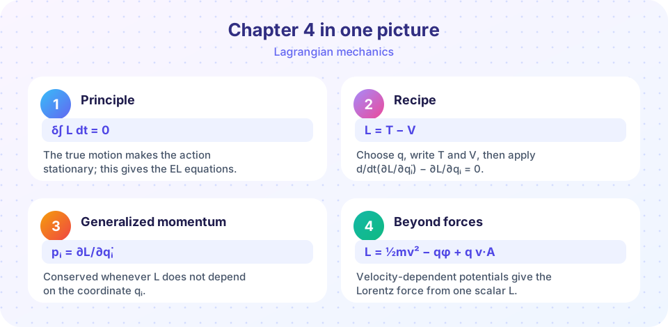
Chapter 4 is the heart of the course. You derived Lagrange's equations from D'Alembert's principle, used them on an Atwood machine and a rotating hoop, defined generalized momentum, and applied a velocity-dependent potential to a charged particle. The poster below summarizes the chapter, the table links ideas to lessons, and the quiz mixes all four lessons.
Recap table
| Idea | Statement | Lesson |
|---|---|---|
| Recipe | choose q, write T, V, L = T − V, apply Lagrange's equations, solve |
Overview |
| Lagrange's equations | d/dt(∂L/∂q̇ⱼ) − ∂L/∂qⱼ = 0 |
Overview |
| D'Alembert | Σ (Fᵃ − m r̈) · δr = 0; constraint forces drop out |
From D'Alembert to Lagrange |
| Generalized force | Qⱼ = Σ F · ∂r/∂qⱼ; drag enters as Qⱼ |
From D'Alembert to Lagrange |
| Atwood machine | ẍ = (m₁ − m₂)g/(m₁ + m₂) |
Worked examples |
| Rotating hoop | θ̈ = sin θ (ω² cos θ − g/R), ω_c = √(g/R) |
Worked examples |
| Generalized momentum | pⱼ = ∂L/∂q̇ⱼ; cyclic coordinate ⇒ pⱼ constant |
Generalized momentum |
| Charged particle | L = ½mv² − qφ + q v·A, p = mv + qA |
Generalized momentum |
Try it
A practice problem with the full recipe in code: a bead of mass m on a frictionless parabolic wire y = a x², with gravity acting downward. One coordinate x suffices.
Press Run (or Ctrl + Enter) to see the result here.
Program input · what you'd type while the program runs
Type the answers before you press Run, one per line. Each time the program reads a line (with input()), it gets the next line from this box.
Press Run (or Ctrl + Enter) to see the result here.
Program input · what you'd type while the program runs
Type the answers before you press Run, one per line. Each time the program reads a line (with input()), it gets the next line from this box.
Check your understanding
Quick check · 10 questions
of 10 answered You scored / 10 · perfect!
-
1. Which statement about Lagrange's equations is correct?
Smooth constraint forces do no virtual work, so they are absent. -
2. In the five-step recipe, which comes immediately after writing T and V?
Choose q, write T and V, form L, apply the equations, solve. -
3. Which is the generalized momentum conjugate to θ for L = ½ m l² θ̇² + m g l cos θ?
pθ = ∂L/∂θ̇ = m l² θ̇. -
4. If a coordinate is cyclic, then:
∂L/∂q = 0 implies dp/dt = 0. -
5. What generalized force represents a viscous drag torque −cθ̇?
The torque is the virtual work per unit δθ. -
6. For the Atwood machine, what is the tension if m₁ = 3 kg and m₂ = 1 kg (g = 9.81 m/s²)?
T = 2 m₁ m₂ g/(m₁ + m₂) = 14.715 N. -
7. The canonical momentum of a charged particle in a vector potential A is:
∂L/∂v = m v + q A. -
8. Above ω_c = √(g/R) the bead on the rotating hoop has new equilibria where:
θ̈ = 0 gives ω² cos θ = g/R. -
9. Which force does no work on a charged particle?
The magnetic force is perpendicular to the velocity. -
10. What is the main advantage of D'Alembert's principle?
Constraint forces are perpendicular to virtual displacements.
Summary
- Lagrange's equations come from D'Alembert's principle or Hamilton's principle; they hold for any generalized coordinates.
- The recipe is mechanical; most effort goes into choosing
qand writingT. - Generalized momentum
pⱼ = ∂L/∂q̇ⱼis conserved for cyclic coordinates. - Velocity-dependent potentials give the Lorentz force and the canonical momentum
m v + q A. - Slice B of the course continues with symmetry and conservation laws, then Hamiltonian mechanics.
Track your progress
Create a free account to tick off lessons and pick up where you left off on any device.
of Classical Mechanics: Lagrangian and Hamiltonian lessons completed